
1.9.14: Exponential and Logarithmic Functions


- Last updated
- May 22, 2025
- Save as PDF

( \newcommand{\kernel}{\mathrm{null}\,}\)
- Identify the form of an exponential function.
- Explain the difference between the graphs of xb and bx.
- Recognize the significance of the number e.
- Identify the form of a logarithmic function.
- Explain the relationship between exponential and logarithmic functions.
- Describe how to calculate a logarithm to a different base.
In this section we examine exponential and logarithmic functions. We use the properties of these functions to solve equations involving exponential or logarithmic terms, and we study the meaning and importance of the number e.
Exponential Functions
Recall the properties of exponents: If x is a positive integer, then we define bx=b⋅b⋯b (with x factors of b). If x is a negative integer, then x=−y for some positive integer y, and we define bx=b−y=1/by. Also, b0 is defined to be 1. If x is a rational number, then x=p/q, where p and q are integers and bx=bp/q=q√bp. For example, 93/2=√93=(√9)3=27.
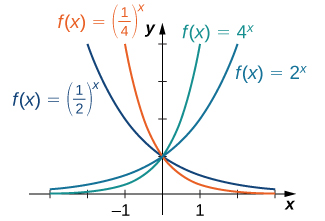
For any base b>0, b≠1, the exponential function f(x)=bx is defined for all real numbers x and bx>0. Therefore, the domain of f(x)=bx is (−∞,∞) and the range is (0,∞). To graph bx, we note that for b>1, bx is increasing on (−∞,∞) and bx→∞ as x→∞, whereas bx→0 as x→−∞. On the other hand, if 0<b<1, f(x)=bx is decreasing on (−∞,∞) and bx→0 as x→∞ whereas bx→∞ as x→−∞ (Figure 1.9.14.2).
Note that exponential functions satisfy the general laws of exponents. To remind you of these laws, we state them as rules.
For any constants a>0, b>0, and for all x and y,
- bx⋅by=bx+y
- bxby=bx−y
- (bx)y=bxy
- (ab)x=axbx
- axbx=(ab)x
Use the laws of exponents to simplify each of the following expressions.
- (2x2/3)3(4x−1/3)2
- (x3y−1)2(xy2)−2
- Solution
-
a. We can simplify as follows:
(2x2/3)3(4x−1/3)2=23(x2/3)342(x−1/3)2=8x216x−2/3=x2x2/32=x8/32.
b. We can simplify as follows:
(x3y−1)2(xy2)−2=(x3)2(y−1)2x−2(y2)−2=x6y−2x−2y−4=x6x2y−2y4=x8y2.
The Number e
A special type of exponential function appears frequently in real-world applications involves the Euler number e:
e≈2.718282.
The letter e was first used to represent this number by the Swiss mathematician Leonhard Euler during the 1720s. Although Euler did not discover the number, he showed many important connections between e and logarithmic functions. We still use the notation e today to honor Euler’s work because it appears in many areas of mathematics and because we can use it in many practical applications.
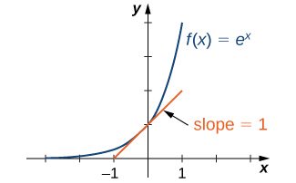
Functions involving base e arise often in applications, we call the function f(x)=ex the natural exponential function. Since e>1, we know f(x)=ex is increasing on (−∞,∞). In Figure 1.9.14.3, we show a graph of f(x)=ex along with a tangent line to the graph of f at x=0. The function f(x)=ex is the only exponential function bx with tangent line at x=0 that has a slope of 1. As we see later in the text, having this property makes the natural exponential function the most simple exponential function to use in many instances.
Logarithmic Functions
Using our understanding of exponential functions, we can discuss their inverses, which are the logarithmic functions. These come in handy when we need to consider any phenomenon that varies over a wide range of values, such as the pH scale in chemistry or decibels in sound levels.
The exponential function f(x)=bx is one-to-one, with domain (−∞,∞) and range (0,∞). Therefore, it has an inverse function, called the logarithmic function with base b. For any b>0,b≠1, the logarithmic function with base b, denoted logb, has domain (0,∞) and range (−∞,∞),and satisfies
logb(x)=y
if and only if by=x.
For example,
log2(8)=3
since 23=8,
log10(1100)=−2
since 10−2=1102=1100,
logb(1)=0
since b0=1 for any base b>0.
Furthermore, since y=logb(x) and y=bx are inverse functions,
logb(bx)=x
and
blogb(x)=x.
The most commonly used logarithmic function is the function loge. Since this function uses natural e as its base, it is called the natural logarithm. Here we use the notation ln(x) or lnx to mean loge(x). For example,
ln(e)=loge(e)=1ln(e3)=loge(e3)=3ln(1)=loge(1)=0.
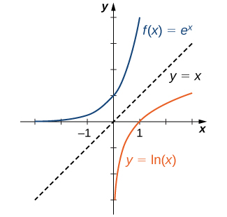
Since the functions f(x)=ex and g(x)=ln(x) are inverses of each other,
ln(ex)=x and elnx=x,
and their graphs are symmetric about the line y=x (Figure 1.9.14.4).
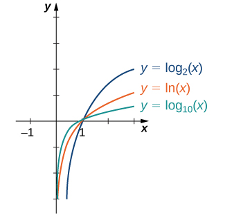
In general, for any base b>0, b≠1, the function g(x)=logb(x) is symmetric about the line y=x with the function f(x)=bx. Using this fact and the graphs of the exponential functions, we graph functions logb for several values of b>1 ( Figure 1.9.14.5).
Before solving some equations involving exponential and logarithmic functions, let’s review the basic properties of logarithms.
If a,b,c>0,b≠1, and r is any real number, then
- Product property
logb(ac)=logb(a)+logb(c)
- Quotient property
logb(ac)=logb(a)−logb(c)
- Power property
logb(ar)=rlogb(a)
Solve each of the following equations for x.
- 5x=2
- ex+6e−x=5
- Solution
-
a. Applying the natural logarithm function to both sides of the equation, we have
ln5x=ln2.
Using the power property of logarithms,
xln5=ln2.
Therefore,
x=ln2ln5.
b. Multiplying both sides of the equation by ex,we arrive at the equation
e2x+6=5ex.
Rewriting this equation as
e2x−5ex+6=0,
we can then rewrite it as a quadratic equation in ex:
(ex)2−5(ex)+6=0.
Now we can solve the quadratic equation. Factoring this equation, we obtain
(ex−3)(ex−2)=0.
Therefore, the solutions satisfy ex=3 and ex=2. Taking the natural logarithm of both sides gives us the solutions x=ln3,ln2.
Solve each of the following equations for x.
- ln(1x)=4
- log10√x+log10x=2
- ln(2x)−3ln(x2)=0
- Solution
-
a. By the definition of the natural logarithm function,
ln(1x)=4
- if and only if e4=1x.
Therefore, the solution is x=1/e4.
b. Using the product (Equation ???) and power (Equation ???) properties of logarithmic functions, rewrite the left-hand side of the equation as
log10√x+log10x=log10x√x=log10x3/2=32log10x.
Therefore, the equation can be rewritten as
32log10x=2
or
log10x=43.
The solution is x=104/3=103√10.
c. Using the power property (Equation ???) of logarithmic functions, we can rewrite the equation as ln(2x)−ln(x6)=0.
Using the quotient property (Equation ???), this becomes
ln(2x5)=0
Therefore, 2/x5=1, which implies x=5√2. We should then check for any extraneous solutions.
When evaluating a logarithmic function with a calculator, you may have noticed that the only options are log10 or log, called the common logarithm, or ln, which is the natural logarithm. However, exponential functions and logarithm functions can be expressed in terms of any desired base b. If you need to use a calculator to evaluate an expression with a different base, you can apply the change-of-base formulas first. Using this change of base, we typically write a given exponential or logarithmic function in terms of the natural exponential and natural logarithmic functions.
Let a>0,b>0, and a≠1,b≠1.
1. ax=bxlogba for any real number x.
If b=e, this equation reduces to ax=exlogea=exlna.
2. logax=logbxlogba for any real number x>0.
If b=e, this equation reduces to logax=lnxlna.
Use a calculating utility to evaluate log37 with the change-of-base formula presented earlier.
- Solution
-
Use the second equation with a=3 and b=e: log37=ln7ln3≈1.77124.
In 1935, Charles Richter developed a scale (now known as the Richter scale) to measure the magnitude of an earthquake. The scale is a base-10 logarithmic scale, and it can be described as follows: Consider one earthquake with magnitude R1 on the Richter scale and a second earthquake with magnitude R2 on the Richter scale. Suppose R1>R2, which means the earthquake of magnitude R1 is stronger, but how much stronger is it than the other earthquake?

A way of measuring the intensity of an earthquake is by using a seismograph to measure the amplitude of the earthquake waves. If A1 is the amplitude measured for the first earthquake and A2 is the amplitude measured for the second earthquake, then the amplitudes and magnitudes of the two earthquakes satisfy the following equation:
R1−R2=log10(A1A2).
Consider an earthquake that measures 8 on the Richter scale and an earthquake that measures 7 on the Richter scale. Then,
8−7=log10(A1A2).
Therefore,
log10(A1A2)=1,
which implies A1/A2=10 or A1=10A2. Since A1 is 10 times the size of A2, we say that the first earthquake is 10 times as intense as the second earthquake. On the other hand, if one earthquake measures 8 on the Richter scale and another measures 6, then the relative intensity of the two earthquakes satisfies the equation
log10(A1A2)=8−6=2.
Therefore, A1=100A2.That is, the first earthquake is 100 times more intense than the second earthquake.
How can we use logarithmic functions to compare the relative severity of the magnitude 9 earthquake in Japan in 2011 with the magnitude 7.3 earthquake in Haiti in 2010?
- Solution
-
To compare the Japan and Haiti earthquakes, we can use an equation presented earlier:
9−7.3=log10(A1A2).
Therefore, A1/A2=101.7, and we conclude that the earthquake in Japan was approximately 50 times more intense than the earthquake in Haiti.
Use the Properties of Logarithms
Now that we have learned about exponential and logarithmic functions, we can introduce some of the properties of logarithms. These will be very helpful as we continue to solve both exponential and logarithmic equations.
The first two properties derive from the definition of logarithms. Since a0=1, we can convert this to logarithmic form and get loga1=0. Also, since a1=a, we get logaa=1.
Properties of Logarithms
loga1=0logaa=1
In the next example we could evaluate the logarithm by converting to exponential form, as we have done previously, but recognizing and then applying the properties saves time.
Evaluate using the properties of logarithms:
- log81
- log66
- Solution
-
a.
log81
Use the property, loga1=0.
0log81=0
b.
log66
Use the property, logaa=1.
1log66=1
The next two properties can also be verified by converting them from exponential form to logarithmic form, or the reverse.
The exponential equation alogax=x converts to the logarithmic equation logax=logax, which is a true statement for positive values for x only.
The logarithmic equation logaax=x converts to the exponential equation ax=ax, which is also a true statement.
These two properties are called inverse properties because, when we have the same base, raising to a power “undoes” the log and taking the log “undoes” raising to a power. These two properties show the composition of functions. Both ended up with the identity function which shows again that the exponential and logarithmic functions are inverse functions.
Inverse Properties of Logarithms
For a>0,x>0 and a≠1,
alogax=xlogaax=x
In the next example, apply the inverse properties of logarithms.
Evaluate using the properties of logarithms:
- 4log49
- log335
- Solution
-
a.
4log49
Use the property, alogax=x.
94log49=9
b.
log335
Use the property, alogax=x.
5log335=5
There are three more properties of logarithms that will be useful in our work. We know exponential functions and logarithmic function are very interrelated. Our definition of logarithm shows us that a logarithm is the exponent of the equivalent exponential. The properties of exponents have related properties for exponents.
In the Product Property of Exponents, am⋅an=am+n, we see that to multiply the same base, we add the exponents. The Product Property of Logarithms, logaM⋅N=logaM+logaN tells us to take the log of a product, we add the log of the factors.
Product Property of Logarithms
If M>0,N>0,a>0 and a≠1, then
loga(M⋅N)=logaM+logaN
The logarithm of a product is the sum of the logarithms.
We use this property to write the log of a product as a sum of the logs of each factor.
Use the Product Property of Logarithms to write each logarithm as a sum of logarithms. Simplify, if possible:
- log37x
- log464xy
- Solution
-
a.
log37x
Use the Product Property, loga(M⋅N)=logaM+logaN.
log37+log3x
log37x=log37+log3xb.
log464xy
Use the Product Property, loga(M⋅N)=logaM+logaN.
log464+log4x+log4y
Simplify be evaluating, log464.
3+log4x+log4y
log464xy=3+log4x+log4y
Similarly, in the Quotient Property of Exponents, aman=am−n, we see that to divide the same base, we subtract the exponents. The Quotient Property of Logarithms, logaMN=logaM−logaN tells us to take the log of a quotient, we subtract the log of the numerator and denominator.
Quotient Property of Logarithms
If M>0,N>0,a>0 and a≠1, then
logaMN=logaM−logaN
The logarithm of a quotient is the difference of the logarithms.
Note that logaM=logaN≠loga(M−N).
We use this property to write the log of a quotient as a difference of the logs of each factor.
Use the Quotient Property of Logarithms to write each logarithm as a difference of logarithms. Simplify, if possible.
- log557
- logx100
- Solution
-
a.
log557
Use the Quotient Property, logaMN=logaM−logaN.
log55−log57
Simplify.
1−log57
log557=1−log57
b.
logx100
Use the Quotient Property, logaMN=logaM−logaN.
logx−log100
Simplify.
logx−2
logx100=logx−2
The third property of logarithms is related to the Power Property of Exponents, (am)n=am⋅n, we see that to raise a power to a power, we multiply the exponents. The Power Property of Logarithms, logaMp=plogaM tells us to take the log of a number raised to a power, we multiply the power times the log of the number.
Power Property of Logarithms
If M>0,a>0,a≠1 and p is any real number then,
logaMp=plogaM
The log of a number raised to a power as the product product of the power times the log of the number.
We use this property to write the log of a number raised to a power as the product of the power times the log of the number. We essentially take the exponent and throw it in front of the logarithm.
Use the Power Property of Logarithms to write each logarithm as a product of logarithms. Simplify, if possible.
- log543
- logx10
- Solution
-
a.
log543
Use the Power Property, logaMp=plogaM.
3 log54
log543=3log54
b.
logx10
Use the Power Property, logaMp=plogaM.
10logx
logx10=10logx
We summarize the Properties of Logarithms here for easy reference. While the natural logarithms are a special case of these properties, it is often helpful to also show the natural logarithm version of each property.
Properties of Logarithms
If M>0,a>0,a≠1 and p is any real number then,
| Property | Base a | Base e |
|---|---|---|
| loga1=0 | ln1=0 | |
| logaa=1 | lne=1 | |
| Inverse Properties | alogax=x logaax=x |
elnx=x lnex=x |
| Product Property of Logarithms | loga(M⋅N)=logaM+logaN | ln(M⋅N)=lnM+lnN |
| Quotient Property of Logarithms | logaMN=logaM−logaN | lnMN=lnM−lnN |
| Power Property of Logarithms | logaMp=plogaM | lnMp=plnM |
Now that we have the properties we can use them to “expand” a logarithmic expression. This means to write the logarithm as a sum or difference and without any powers.
We generally apply the Product and Quotient Properties before we apply the Power Property.
Use the Properties of Logarithms to expand the logarithm log4(2x3y2). Simplify, if possible.
- Solution
-
Use the Product Property, logaM⋅N=logaM+logaN.
Use the Power Property, logaMp=plogaM, on the last two terms. Simplify.
When we have a radical in the logarithmic expression, it is helpful to first write its radicand as a rational exponent.
Use the Properties of Logarithms to expand the logarithm log24√x33y2z. Simplify, if possible.
- Solution
-
log24√x33y2z
Rewrite the radical with a rational exponent.
log2(x33y2z)14
Use the Power Property, logaMp=plogaM.
14log2(x33y2z)
Use the Quotient Property, logaM⋅N=logaM−logaN.
14(log2(x3)−log2(3y2z))
Use the Product Property, logaM⋅N=logaM+logaN, in the second term.
14(log2(x3)−(log23+log2y2+log2z))
Use the Power Property, logaMp=plogaM, inside the parentheses.
14(3log2x−(log23+2log2y+log2z))
Simplify by distributing.
14(3log2x−log23−2log2y−log2z)
log24√x33y2z=14(3log2x−log23−2log2y−log2z)
The opposite of expanding a logarithm is to condense a sum or difference of logarithms that have the same base into a single logarithm. We again use the properties of logarithms to help us, but in reverse.
To condense logarithmic expressions with the same base into one logarithm, we start by using the Power Property to get the coefficients of the log terms to be one and then the Product and Quotient Properties as needed.
Use the Properties of Logarithms to condense the logarithm log43+log4x−log4y. Simplify, if possible.
- Solution
-
The log expressions all have the same base, 4.
The first two terms are added, so we use the Product Property, logaM+logaN=logaM:N.
Since the logs are subtracted, we use the Quotient Property, logaM−logaN=logaMN.
Use the Properties of Logarithms to condense the logarithm 2log3x+4log3(x+1). Simplify, if possible.
- Solution
-
The log expressions have the same base, 3.
2log3x+4log3(x+1)
Use the Power Property, logaM+logaN=logaM⋅N.
log3x2+log3(x+1)4
The terms are added, so we use the Product Property, logaM+logaN=logaM⋅N.
log3x2(x+1)4
2log3x+4log3(x+1)=log3x2(x+1)4
Use the Change-of-Base Formula
To evaluate a logarithm with any other base, we can use the Change-of-Base Formula. We will show how this is derived.
Suppose we want to evaluatelogaMlogaMLety=logaM.y=logaMRewrite the epression in exponential form. ay=MTake the logbof each side.logbay=logbMUse the Power Property.ylogba=logbMSolve fory.y=logbMlogbaSubstiturey=logaM.logaM=logbMlogba
The Change-of-Base Formula introduces a new base b. This can be any base b we want where b>0,b≠1. Because our calculators have keys for logarithms base 10 and base e, we will rewrite the Change-of-Base Formula with the new base as 10 or e.
Change-of-Base Formula
For any logarithmic bases a,b and M>0,
logaM=logbMlogbalogaM=logMlogalogaM=lnMlna new base b new base 10 new base e
When we use a calculator to find the logarithm value, we usually round to three decimal places. This gives us an approximate value and so we use the approximately equal symbol (≈).
Rounding to three decimal places, approximate log435.
- Solution
-

Use the Change-of-Base Formula. 
Identify a and M. Choose 10 for b. 
Enter the expression log35log4 in the calculator using the log button for base 10. Round to three decimal places. 
Table 10.4.2
In the previous section, we derived two important properties of logarithms, which allowed us to solve some basic exponential and logarithmic equations.
Inverse Properties:
logb(bx)=x
blogbx=x
Exponential Property:
logb(Ar)=rlogb(A)
Change of Base:
logb(A)=logc(A)logc(b)
While these properties allow us to solve a large number of problems, they are not sufficient to solve all problems involving exponential and logarithmic equations.
Sum of Logs Property:
logb(A)+logb(C)=logb(AC)
Difference of Logs Property:
logb(A)−logb(C)=logb(AC)
It’s just as important to know what properties logarithms do not satisfy as to memorize the valid properties listed above. In particular, the logarithm is not a linear function, which means that it does not distribute:
logA+B≠logA+logB.
To help in this process we offer a proof of Equation ??? to help solidify our new rules and show how they follow from properties you’ve already seen.
Let a=logb(A) and c=logb(C).
By definition of the logarithm, ba=A and bc=C.
Using these expressions,
AC=babc
Using exponent rules on the right,
AC=ba+c
Taking the log of both sides, and utilizing the inverse property of logs,
logb(AC)=logb(ba+c)=a+c
Replacing a and c with their definition establishes the result
logb(AC)=logbA+logbC
The proof for the difference property is very similar.
With these properties, we can rewrite expressions involving multiple logs as a single log, or break an expression involving a single log into expressions involving multiple logs.
Write log3(5)+log3(8)−log3(2) as a single logarithm.
- Solution
-
Using the sum of logs property on the first two terms,
log3(5)+log3(8)=log3(5⋅8)=log3(40)
This reduces our original expression to
log3(40)−log3(2)
Then using the difference of logs property,
log3(40)−log3(2)=log3(402)=log3(20)
Evaluate 2log(5)+log(4) without a calculator by first rewriting as a single logarithm.
- Solution
-
On the first term, we can use the exponent property of logs to write
2log(5)=log(52)=log(25)
With the expression reduced to a sum of two logs, log(25)+log(4), we can utilize the sum of logs property
log(25)+log(4)=log(4⋅25)=log(100)
Since 100=102, we can evaluate this log without a calculator:
log(100)=log(102)=2
Rewrite ln(x4y7) as a sum or difference of logs
- Solution
-
First, noticing we have a quotient of two expressions, we can utilize the difference property of logs to write
ln(x4y7)=ln(x4y)−ln(7)
Then seeing the product in the first term, we use the sum property
ln(x4y)−ln(7)=ln(x4)+ln(y)−ln(7)
Finally, we could use the exponent property on the first term
ln(x4)+ln(y)−ln(7)=4ln(x)+ln(y)−ln(7)
Log properties in Solving Equations
The logarithm properties often arise when solving problems involving logarithms. First, we’ll look at a simpler log equation.
Solve log(2x−6)=3.
- Solution
-
To solve for x, we need to get it out from inside the log function. There are two ways we can approach this.
Method 1: Rewrite as an exponential.
Recall that since the common log is base 10, log(A)=B can be rewritten as the exponential 10B=A. Likewise, log(2x−6)=3 can be rewritten in exponential form as
103=2x−6
Method 2: Exponentiate both sides.
If A=B, then 10A=10B. Using this idea, since log(2x−6)=3, then 10log(2x−6)=103. Use the inverse property of logs to rewrite the left side and get 2x−6=103.
Using either method, we now need to solve 2x−6=103. Evaluate 103 to get
2x−6=1000 Add 6 to both sides
2x=1006 Divide both sides by 2
x=503Occasionally the solving process will result in extraneous solutions – answers that are outside the domain of the original equation. In this case, our answer looks fine.
Solve log(50x+25)−log(x)=2.
- Solution
-
In order to rewrite in exponential form, we need a single logarithmic expression on the left side of the equation. Using the difference property of logs, we can rewrite the left side:
log(50x+25x)=2
Rewriting in exponential form reduces this to an algebraic equation:
50x+25x=102=100 Multiply both sides by x
50x+25=100x Combine like terms
25=50x Divide by 50
x=2550=12Checking this answer in the original equation, we can verify there are no domain issues, and this answer is correct.
Solve ln(x+2)+ln(x+1)=ln(4x+14).
- Solution
-
ln(x+2)+ln(x+1)=ln(4x+14) Use the sum of logs property on the right
ln((x+2)(x+1))=ln(4x+14) Expand
ln(x2+3x+2)=ln(4x+14)We have a log on both side of the equation this time. Rewriting in exponential form would be tricky, so instead we can exponentiate both sides.
eln(x2+3x+2)=eln(4x+13) Use the inverse property of logs
x2+3x+2=4x+14 Move terms to one side
x2−x−12=0 Factor
(x+4)(x−3)=0
x=−4 or x=3Checking our answers, notice that evaluating the original equation at x=−4 would result in us evaluating ln(−2), which is undefined. That answer is outside the domain of the original equation, so it is an extraneous solution and we discard it. There is one solution: x=3.
More complex exponential equations can often be solved in more than one way. In the following example, we will solve the same problem in two ways – one using logarithm properties, and the other using exponential properties.
In 2008, the population of Kenya was approximately 38.8 million, and was growing by 2.64% each year, while the population of Sudan was approximately 41.3 million and growing by 2.24% each year(World Bank, World Development Indicators, as reported on http://www.google.com/publicdata, retrieved August 24, 2010). If these trends continue, when will the population of Kenya match that of Sudan?
- Solution
-
We start by writing an equation for each population in terms of t, the number of years after 2008.
Kenya(t)=38.8(1+0.0264)tSudan(t)=41.3(1+0.0224)t
To find when the populations will be equal, we can set the equations equal
38.8(1.0264)t=41.3(1.0224)t
For our first approach, we take the log of both sides of the equation.
log(38.8(1.0264)t)=log(41.3(1.0224)t)
Utilizing the sum property of logs, we can rewrite each side,
log(38.8)+log(1.0264t)=log(41.3)+log(1.0224t)
Then utilizing the exponent property, we can pull the variables out of the exponent
log(38.8)+tlog(1.0264)=log(41.3)+tlog(1.0224)
Moving all the terms involving t to one side of the equation and the rest of the terms to the other side,
tlog(1.0264)−tlog(1.0224)=log(41.3)−log(38.8)
Factoring out the t on the left,
t(log(1.0264)−log(1.0224))=log(41.3)−log(38.8)
Dividing to solve for t
t=log(41.3)−log(38.8)log(1.0264)−log(1.0224)≈15.991
It will be 15.991 years until the populations will be equal.
Solve the problem above by rewriting before taking the log.
- Solution
-
Starting at the equation
38.8(1.0264)t=41.3(1.0224)t
Divide to move the exponential terms to one side of the equation and the constants to the other side
1.0264t1.0224t=41.338.8
Using exponent rules to group on the left,
(1.02641.0224)t=41.338.8
Taking the log of both sides
log((1.02641.0224)t)=log(41.338.8)
Utilizing the exponent property on the left,
tlog(1.02641.0224)=log(41.338.8)
Dividing gives
t=log(41.338.8)log(1.02641.0224)≈15.991 years
While the answer does not immediately appear identical to that produced using the previous method, note that by using the difference property of logs, the answer could be rewritten:
t=log(41.338.8)log(1.02641.0224)=log(41.3)−log(38.8)log(1.0264)−log(1.0224)
While both methods work equally well, it often requires fewer steps to utilize algebra before taking logs, rather than relying solely on log properties.
Applications
While we have explored some basic applications of exponential and logarithmic functions, in this section we explore some important applications in more depth.
Radioactive Decay
In Nuclear Physics we discuss radioactive decay – the idea that radioactive isotopes change over time. One of the common terms associated with radioactive decay is half-life.
The half-life of a radioactive isotope is the time it takes for half the substance to decay.
Given the basic exponential growth/decay equation h(t)=abt, half-life can be found by solving for when half the original amount remains; by solving 12a=a(b)t, or more simply 12=bt. Notice how the initial amount is irrelevant when solving for half-life.
Bismuth-210 is an isotope that decays by about 13% each day. What is the half-life of Bismuth-210?
- Solution
-
We were not given a starting quantity, so we could either make up a value or use an unknown constant to represent the starting amount. To show that starting quantity does not affect the result, let us denote the initial quantity by the constant a. Then the decay of Bismuth-210 can be described by the equation Q(d)=a(0.87)d.
To find the half-life, we want to determine when the remaining quantity is half the original: 12a. Solving,
12a=a(0.87)d Divide by a,
12=0.87d Take the log of both sides
log(12)=log(0.87d) Use the exponent property of logs
log(12)=dlog(0.87) Divide to solve for d
d=log(12)log(0.87)≈4.977 days
This tells us that the half-life of Bismuth-210 is approximately 5 days.
Cesium-137 has a half-life of about 30 years. If you begin with 200 mg of cesium-137, how much will remain after 30 years? 60 years? 90 years?
- Solution
-
Since the half-life is 30 years, after 30 years, half the original amount, 100 mg, will remain.
After 60 years, another 30 years have passed, so during that second 30 years, another half of the substance will decay, leaving 50 mg.
After 90 years, another 30 years have passed, so another half of the substance will decay, leaving 25 mg.
Cesium-137 has a half-life of about 30 years. Find the annual decay rate.
- Solution
-
Since we are looking for an annual decay rate, we will use an equation of the form Q(t)=a(1+r)t. We know that after 30 years, half the original amount will remain. Using this information
12a=a(1+r)30 Dividing by a
12=(1+r)30 Taking the 30th root of both sides
30√12=1+r Subtracting one from both sides,
r=30√12−1≈−0.02284
This tells us cesium-137 is decaying at an annual rate of 2.284% per year.
Carbon-14 is a radioactive isotope that is present in organic materials, and is commonly used for dating historical artifacts. Carbon-14 has a half-life of 5730 years. If a bone fragment is found that contains 20% of its original carbon-14, how old is the bone?
- Solution
-
To find how old the bone is, we first will need to find an equation for the decay of the carbon-14. We could either use a continuous or annual decay formula, but opt to use the continuous decay formula since it is more common in scientific texts. The half life tells us that after 5730 years, half the original substance remains. Solving for the rate,
12a=aer5730 Dividing by a
12=er5730 Taking the natural log of both sides
ln(12)=ln(er5730) Use the inverse property of logs on the right side
ln(12)=5730r Divide by 5730
r=ln(12)5730≈−0.000121
Now we know the decay will follow the equation Q(t)=ae−0.000121t. To find how old the bone fragment is that contains 20% of the original amount, we solve for t so that Q(t)=0.20a.
0.20a=ae−0.000121t
0.20=e−0.000121t
ln(0.20)=ln(e−0.000121t)
ln(0.20)=−0.000121t
t=ln(0.20)−0.000121≈13301 yearsThe bone fragment is about 13,300 years old.
Doubling Time
For decaying quantities, we asked how long it takes for half the substance to decay. For growing quantities we might ask how long it takes for the quantity to double.
The doubling time of a growing quantity is the time it takes for the quantity to double.
Given the basic exponential growth equation h(t)=abt, doubling time can be found by solving for when the original quantity has doubled; by solving 2a=a(b)x, or more simply 2=bx. Like with decay, the initial amount is irrelevant when solving for doubling time.
Cancer cells sometimes increase exponentially. If a cancerous growth contained 300 cells last month and 360 cells this month, how long will it take for the number of cancer cells to double?
- Solution
-
Defining t to be time in months, with t=0 corresponding to this month, we are given two pieces of data: this month, (0, 360), and last month, (-1, 300).
From this data, we can find an equation for the growth. Using the form C(t)=abt, we know immediately a = 360, giving C(t)=360bt. Substituting in (-1, 300), 300=360b−1300=360bb=360300=1.2
This gives us the equation C(t)=360(1.2)t
To find the doubling time, we look for the time when we will have twice the original amount, so when C(t)=2a.
2a=a(1.2)t
2=(1.2)t
log(2)=log(1.2t)
log(2)=tlog(1.2)
t=log(2)log(1.2)≈3.802 months for the number of cancer cells to double.
Use of a new social networking website has been growing exponentially, with the number of new members doubling every 5 months. If the site currently has 120,000 users and this trend continues, how many users will the site have in 1 year?
- Solution
-
We can use the doubling time to find a function that models the number of site users, and then use that equation to answer the question. While we could use an arbitrary a as we have before for the initial amount, in this case, we know the initial amount was 120,000.
If we use a continuous growth equation, it would look like N(t)=120ert, measured in thousands of users after t months. Based on the doubling time, there would be 240 thousand users after 5 months. This allows us to solve for the continuous growth rate:
240=120er5
2=er5
ln2=5r
r=ln25≈0.1386Now that we have an equation, N(t)=120e0.1386t, we can predict the number of users after 12 months:
N(12)=120e0.1386(12)=633.140 thousand users.
So after 1 year, we would expect the site to have around 633,140 users.
Newton’s Law of Cooling
When a hot object is left in surrounding air that is at a lower temperature, the object’s temperature will decrease exponentially, leveling off towards the surrounding air temperature. This "leveling off" will correspond to a horizontal asymptote in the graph of the temperature function. Unless the room temperature is zero, this will correspond to a vertical shift of the generic exponential decay function.
The temperature of an object, T, in surrounding air with temperature Ts will behave according to the formula
T(t)=aekt+Ts
Where
- t is time
- a is a constant determined by the initial temperature of the object
- k is a constant, the continuous rate of cooling of the object
While an equation of the form T(t)=abt+Ts could be used, the continuous growth form is more common.
A cheesecake is taken out of the oven with an ideal internal temperature of 165 degrees Fahrenheit, and is placed into a 35 degree refrigerator. After 10 minutes, the cheesecake has cooled to 150 degrees. If you must wait until the cheesecake has cooled to 70 degrees before you eat it, how long will you have to wait?
- Solution
-
Since the surrounding air temperature in the refrigerator is 35 degrees, the cheesecake’s temperature will decay exponentially towards 35, following the equation
T(t)=aekt+35
We know the initial temperature was 165, so T(0)=165. Substituting in these values,
165=aek0+35165=a+35a=130
We were given another pair of data, T(10)=150, which we can use to solve for k
150=130ek10+35
115=130ek10115130=e10kln(115130)=10kk=ln(115130)10=−0.0123Together this gives us the equation for cooling: T(t)=130e−0.0123t+35
Now we can solve for the time it will take for the temperature to cool to 70 degrees.
70=130e−0.0123t+35
35=130e−0.0123t
35130=e−0.0123t
ln(35130)=−0.0123t
t=ln(35130)−0.0123≈106.68It will take about 107 minutes, or one hour and 47 minutes, for the cheesecake to cool. Of course, if you like your cheesecake served chilled, you’d have to wait a bit longer.
Logarithmic Scales
For quantities that vary greatly in magnitude, a standard scale of measurement is not always effective, and utilizing logarithms can make the values more manageable. For example, if the average distances from the sun to the major bodies in our solar system are listed, you see they vary greatly.
| Planet | Distance (millions of km) |
| Mercury | 58 |
| Venus | 108 |
| Earth | 150 |
| Mars | 228 |
| Jupiter | 779 |
| Saturn | 1430 |
| Uranus | 2880 |
| Neptune | 4500 |
Placed on a linear scale – one with equally spaced values – these values get bunched up.
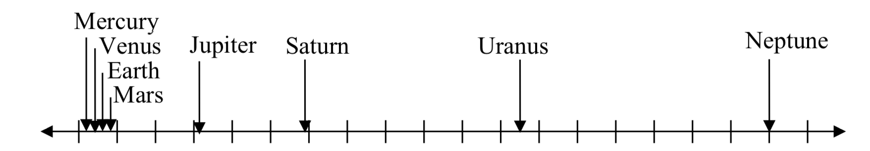
0 500 1000 1500 2000 2500 3000 3500 4000 4500
However, computing the logarithm of each value and plotting these new values on a number line results in a more manageable graph, and makes the relative distances more apparent.(It is interesting to note the large gap between Mars and Jupiter on the log number line. The asteroid belt is located there, which scientists believe is a planet that never formed because of the effects of the gravity of Jupiter.)
| Planet | Distance (millions of km) | log(distance) |
| Mercury | 58 | 1.76 |
| Venus | 108 | 2.03 |
| Earth | 150 | 2.18 |
| Mars | 228 | 2.36 |
| Jupiter | 779 | 2.89 |
| Saturn | 1430 | 3.16 |
| Uranus | 2880 | 3.46 |
| Neptune | 4500 | 3.65 |
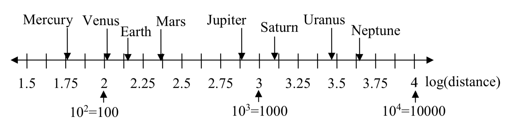
Sometimes, as shown above, the scale on a logarithmic number line will show the log values, but more commonly the original values are listed as powers of 10, as shown below.
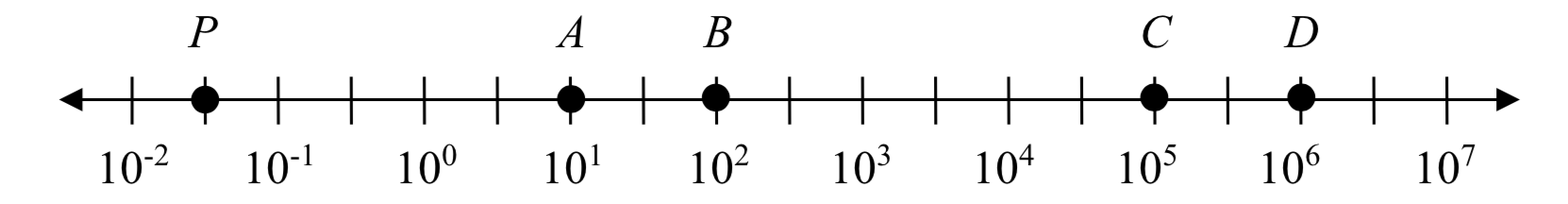
Estimate the value of point P on the log scale above
The point P appears to be half way between -2 and -1 in log value, so if V is the value of this point,
log(V)≈−1.5 Rewriting in exponential form,
V≈10−1.5=0.0316
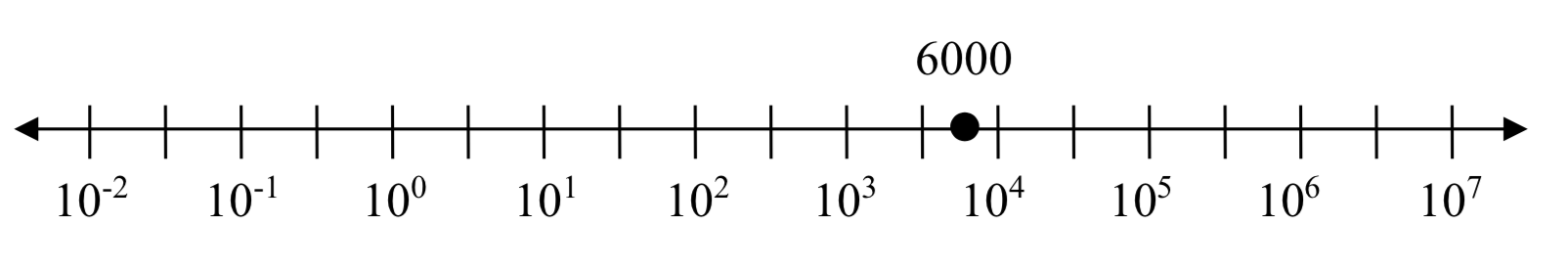
Place the number 6000 on a logarithmic scale.
- Solution
-
Since log(6000)≈3.8, this point would belong on the log scale about here:
Notice that on the log scale above Example 8, the visual distance on the scale between points A and B and between C and D is the same. When looking at the values these points correspond to, notice B is ten times the value of A, and D is ten times the value of C. A visual linear difference between points corresponds to a relative (ratio) change between the corresponding values.
Logarithms are useful for showing these relative changes. For example, comparing $1,000,000 to $10,000, the first is 100 times larger than the second.
1,000,00010,000=100=102
Likewise, comparing $1000 to $10, the first is 100 times larger than the second.
1,00010=100=102
When one quantity is roughly ten times larger than another, we say it is one order of magnitude larger. In both cases described above, the first number was two orders of magnitude larger than the second.
Notice that the order of magnitude can be found as the common logarithm of the ratio of the quantities. On the log scale above, B is one order of magnitude larger than A, and D is one order of magnitude larger than C.
Given two values A and B, to determine how many orders of magnitude A is greater than B,
Difference in orders of magnitude = log(AB)
On the log scale above Example 8, how many orders of magnitude larger is C than B?
- Solution
-
The value B corresponds to 102=100
The value C corresponds to 105=100,000
The relative change is 100,000100=1000=105102=103. The log of this value is 3.
C is three orders of magnitude greater than B, which can be seen on the log scale by the visual difference between the points on the scale.
Earthquakes
An example of a logarithmic scale is the Moment Magnitude Scale (MMS) used for earthquakes. This scale is commonly and mistakenly called the Richter Scale, which was a very similar scale succeeded by the MMS.
For an earthquake with seismic moment S, a measurement of earth movement, the MMS value, or magnitude of the earthquake, is
M=23log(SS0)
Where S0=1016 is a baseline measure for the seismic moment.
If one earthquake has a MMS magnitude of 6.0, and another has a magnitude of 8.0, how much more powerful (in terms of earth movement) is the second earthquake?
- Solution
-
Since the first earthquake has magnitude 6.0, we can find the amount of earth movement for that quake, which we'll denote S1. The value of S0 is not particularity relevant, so we will not replace it with its value.
6.0=23log(S1S0)
6.0(32=log(S1S0)
9=log(S1S0)
S1S0=109
S1=109S0This tells us the first earthquake has about 109 times more earth movement than the baseline measure.
Doing the same with the second earthquake, S2, with a magnitude of 8.0,
8.0=23log(S2S0)
S2=1012S0Comparing the earth movement of the second earthquake to the first,
S2S1=1012S0109S0=103=1000
The second value's earth movement is 1000 times as large as the first earthquake.
One earthquake has magnitude of 3.0. If a second earthquake has twice as much earth movement as the first earthquake, find the magnitude of the second quake.
- Solution
-
Since the first quake has magnitude 3.0,
3.0=23log(SS0)
Solving for S,
3.032=log(SS0)
4.5=log(SS0)
104.5=SS0
S=104.5S0Since the second earthquake has twice as much earth movement, for the second quake,
S=2⋅104.5S0
Finding the magnitude,
M=23log(2⋅104.5S0S0)
M=23log(2⋅104.5)≈3.201The second earthquake with twice as much earth movement will have a magnitude of about 3.2.
In fact, using log properties, we could show that whenever the earth movement doubles, the magnitude will increase by about 0.201:
M=23log(2SS0)=23log(2⋅SS0)
M=23(log(2)+log(SS0))
M=23log(2)+23log(SS0)
M=0.201+23log(SS0)
This illustrates the most important feature of a log scale: that multiplying the quantity being considered will add to the scale value, and vice versa.
Key Concepts
- loga1=0logaa=1
- Inverse Properties of Logarithms
- For a>0,x>0 and a≠1
alogax=xlogaax=x
- For a>0,x>0 and a≠1
- Product Property of Logarithms
- If M>0,N>0,a>0 and a≠1, then,
logaM⋅N=logaM+logaN
The logarithm of a product is the sum of the logarithms.
- If M>0,N>0,a>0 and a≠1, then,
- Quotient Property of Logarithms
- If M>0,N>0,a>0 and a≠1, then,
logaMN=logaM−logaN
The logarithm of a quotient is the difference of the logarithms.
- If M>0,N>0,a>0 and a≠1, then,
- Power Property of Logarithms
- If M>0,a>0,a≠1 and p is any real number then,
logaMp=plogaM
The log of a number raised to a power is the product of the power times the log of the number.
- If M>0,a>0,a≠1 and p is any real number then,
- Properties of Logarithms Summary
If M>0,a>0,a≠1 and p is any real number then,
| Property | Base a | Base e |
|---|---|---|
| loga1=0 | ln1=0 | |
| logaa=1 | lne=1 | |
| Inverse Properties | alogax=x logaax=x |
elnx=x lnex=x |
| Product Property of Logarithms | loga(M⋅N)=logaM+logaN | ln(M⋅N)=lnM+lnN |
| Quotient Property of Logarithms | logaMN=logaM−logaN | lnMN=lnM−lnN |
| Power Property of Logarithms | logaMp=plogaM | lnMp=plnM |
- Change-of-Base Formula
For any logarithmic bases a and b, and M>0,logaM=logbMlogbalogaM=logMlogalogaM=lnMlna new base b new base 10 new base e
Key Concepts
- The exponential function y=bx is increasing if b>1 and decreasing if 0<b<1. Its domain is (−∞,∞) and its range is (0,∞).
- The logarithmic function y=logb(x) is the inverse of y=bx. Its domain is (0,∞) and its range is (−∞,∞).
- The natural exponential function is y=ex and the natural logarithmic function is y=lnx=logex.
- Given an exponential function or logarithmic function in base a, we can make a change of base to convert this function to any base b>0, b≠1. We typically convert to base e.