5.9: Common Forces - Magnetic Force

Learning Objectives

By the end of this section, you will be able to:

• Define the magnetic field based on a moving charge experiencing a force
• Apply the right-hand rule to determine the direction of a magnetic force based on the motion of a charge in a magnetic field
• Explain how a charged particle in an external magnetic field undergoes circular motion
• Describe how to determine the radius of the circular motion of a charged particle in a magnetic field
• Sketch magnetic field lines to understand which way the magnetic field points and how strong it is in a region of space

Magnetism has been known since the time of the ancient Greeks, but it has always been a bit mysterious. You can see electricity in the flash of a lightning bolt, but when a compass needle points to magnetic north, you can’t see any force causing it to rotate. People learned about magnetic properties gradually, over many years, before several physicists of the nineteenth century connected magnetism with electricity.

Defining the Magnetic Field

A magnetic field is defined by the force that a charged particle experiences moving in this field, after we account for the gravitational and any additional electric forces possible on the charge. The magnitude of this force is proportional to the amount of charge q, the speed of the charged particle v, and the magnitude of the applied magnetic field. The direction of this force is perpendicular to both the direction of the moving charged particle and the direction of the applied magnetic field. Based on these observations, we define the magnetic field strength B based on the magnetic force \(\vec{F}\) on a charge q moving at velocity as the cross product of the velocity and magnetic field, that is,

\[\vec{F} = q\vec{v} \times \vec{B}. \label{eq1}\]

In fact, this is how we define the magnetic field \(\vec{B}\) - in terms of the force on a charged particle moving in a magnetic field. The magnitude of the force is determined from the definition of the cross product as it relates to the magnitudes of each of the vectors. In other words, the magnitude of the force satisfies

\[F = qv \, B \sin \, \theta \label{eq2}\]

where θ is the angle between the velocity and the magnetic field.

The SI unit for magnetic field strength \(B\) is called the tesla (T) after the eccentric, but brilliant inventor Nikola Tesla (1856–1943), where

\[1 \, T = \frac{1 \, N}{A \cdot m}.\]

A smaller unit, called the gauss (G) is sometimes used, where

\[1 \, G = 10^{-4} \,T\]

The strongest permanent magnets have fields near 2 T; superconducting electromagnets may attain 10 T or more. Earth’s magnetic field on its surface is only about \(5 \times 10^{-5}\, T\) or \(0.5 \,G\).

Direction of the Magnetic Field by the Right-Hand Rule

The direction of the magnetic force \(\vec{F}\) is perpendicular to the plane formed by \(\vec{v}\) and \(\vec{B}\) as determined by the right-hand rule-1 (or RHR-1), which is illustrated in Figure \(\PageIndex{1}\).

1. Orient your right hand so that your fingers curl in the plane defined by the velocity and magnetic field vectors.
2. Using your right hand, sweep from the velocity toward the magnetic field with your fingers through the smallest angle possible.
3. The magnetic force is directed where your thumb is pointing.
4. If the charge was negative, reverse the direction found by these steps.

   

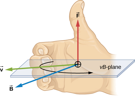
   Figure \(\PageIndex{1}\): Magnetic fields exert forces on moving charges. The direction of the magnetic force on a moving charge is perpendicular to the plane formed by b\(\vec{v}\) and \(\vec{B}\) and follows the right-hand rule-1 (RHR-1) as shown. The magnitude of the force is proportional to \(q, \, v, \, B,\) and the sine of the angle between \(\vec{v}\) and \(\vec{B}\).

There is no magnetic force on static charges. However, there is a magnetic force on charges moving at an angle to a magnetic field. When charges are stationary, their electric fields do not affect magnets. However, when charges move, they produce magnetic fields that exert forces on other magnets. When there is relative motion, a connection between electric and magnetic forces emerges - each affects the other.

Example \(\PageIndex{1}\): An Alpha-Particle Moving in a Magnetic Field

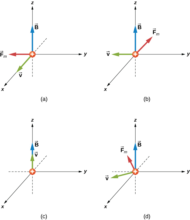
An alpha-particle \((q = 3.2 \times 10^{-19}C)\) moves through a uniform magnetic field whose magnitude is 1.5 T. The field is directly parallel to the positive z-axis of the rectangular coordinate system of Figure \(\PageIndex{2}\). What is the magnetic force on the alpha-particle when it is moving (a) in the positive x-direction with a speed of \(5.0 \times 10^4 m/s\)? (b) in the negative y-direction with a speed of \(5.0 \times 10^4 m/s\)? (c) in the positive z-direction with a speed of \(5.0 \times 10^4 m/s\)? (d) with a velocity \(\vec{v} = \left(2.0 \hat{i} - 3.0 \hat{j} + 1.0 \hat{k} \right) \times 10^4 m/s\)?

Figure \(\PageIndex{2}\): The magnetic forces on an alpha-particle moving in a uniform magnetic field. The field is the same in each drawing, but the velocity is different.

Strategy

We are given the charge, its velocity, and the magnetic field strength and direction. We can thus use the equation \(\vec{F} = q \vec{v} \times \vec{B}\) or \(F = qv \, B sin\, \theta\) to calculate the force. The direction of the force is determined by RHR-1.

Solution

1. First, to determine the direction, start with your fingers pointing in the positive x-direction. Sweep your fingers upward in the direction of magnetic field. Your thumb should point in the negative y-direction. This should match the mathematical answer. To calculate the force, we use the given charge, velocity, and magnetic field and the definition of the magnetic force in cross-product form to calculate: \[\vec{F} = q\vec{v} \times \vec{B} = (3.2 \times 10^{-19} C) (5.0 \times 10^4 m/s \, \hat{i}) \times (1.5 \, T \, \hat{k}) = - 2.4 \times 10^{-14} N \, \hat{j}\]
2. First, to determine the directionality, start with your fingers pointing in the negative y-direction. Sweep your fingers upward in the direction of magnetic field as in the previous problem. Your thumb should be open in the negative x-direction. This should match the mathematical answer. To calculate the force, we use the given charge, velocity, and magnetic field and the definition of the magnetic force in cross-product form to calculate: \[\vec{F} = q\vec{v} \times \vec{B} = (3.2 \times 10^{-19} C) (- 5.0 \times 10^4 m/s \, \hat{i}) \times (1.5 \, T \, \hat{k}) = - 2.4 \times 10^{-14} N \, \hat{i}\] An alternative approach is to use Equation \ref{eq2} to find the magnitude of the force. This applies for both parts (a) and (b). Since the velocity is perpendicular to the magnetic field, the angle between them is 90 degrees. Therefore, the magnitude of the force is: \[F = qv \, B \sin \, \theta = (3.2 \times 10^{-19} C)(5.0 \times 10^4m/s)(1.5 \, T) sin (90^o)) = 2.4 \times 10^{-14} N.\]
3. Since the velocity and magnetic field are parallel to each other, there is no orientation of your hand that will result in a force direction. Therefore, the force on this moving charge is zero. This is confirmed by the cross product. When you cross two vectors pointing in the same direction, the result is equal to zero.
4. First, to determine the direction, your fingers could point in any orientation; however, you must sweep your fingers upward in the direction of the magnetic field. As you rotate your hand, notice that the thumb can point in any x- or y-direction possible, but not in the z-direction. This should match the mathematical answer. To calculate the force, we use the given charge, velocity, and magnetic field and the definition of the magnetic force in cross-product form to calculate: \[\vec{F} = q\vec{v} \times \vec{B} = (3.2 \times 10^{-19} C)((2.0 \hat{i} - 3.0 \hat{j} + 1.0 \hat{k}) \times 10^4 m/s) \times (1.5 \, T \hat{k})\] \[(-14.4 \hat{i} - 9.6 \hat{j}) \times 10^{-15}N.\] This solution can be rewritten in terms of a magnitude and angle in the xy-plane: \[|\vec{F}| = \sqrt{F_x^2 + F_y^2} = \sqrt{(-14.4)^2 + (-9.6)^2} \times 10^{-15} N = 1.7 \times 10^{-14}N\] \[\theta = tan^{-1} \left(\frac{F_y}{F_x}\right) = tan^{-1} \left(\frac{-9.6 \times 10^{-15}N}{-14.4 \times 10^{-15}N} \right) = 34^o.\] The magnitude of the force can also be calculated using Equation \ref{eq2}. The velocity in this question, however, has three components. The z-component of the velocity can be neglected, because it is parallel to the magnetic field and therefore generates no force. The magnitude of the velocity is calculated from the x- and y-components. The angle between the velocity in the xy-plane and the magnetic field in the z-plane is 90 degrees. Therefore, the force is calculated to be: \[|\vec{v}| = \sqrt{(2)^2 + (-3)^2} \times 10^4 \frac{m}{s} = 3.6 \times 10^4 \frac{m}{s}\]\[F = qv \, Bsin \, \theta = (3.2 \times 10^{-19}C)(3.6 \times 10^4 m/s) (1.5 \, T) sin (90^o) = 1.7 \times 10^{-14} N\]

This is the same magnitude of force calculated by unit vectors.

Significance

The cross product in this formula results in a third vector that must be perpendicular to the other two. Other physical quantities, such as angular momentum, also have three vectors that are related by the cross product. Note that typical force values in magnetic force problems are much larger than the gravitational force. Therefore, for an isolated charge, the magnetic force is the dominant force governing the charge’s motion.

Examples of Magnetic Forces

A charged particle experiences a force when moving through a magnetic field. What happens if this field is uniform over the motion of the charged particle? What path does the particle follow? In this section, we discuss the circular motion of the charged particle as well as other motion that results from a charged particle entering a magnetic field.

The simplest case occurs when a charged particle moves perpendicular to a uniform B-field (Figure \(\PageIndex{1}\)). If the field is in a vacuum, the magnetic field is the dominant factor determining the motion. Since the magnetic force is perpendicular to the direction of travel, a charged particle follows a curved path in a magnetic field. The particle continues to follow this curved path until it forms a complete circle. Another way to look at this is that the magnetic force is always perpendicular to velocity, so that it does no work on the charged particle. The particle’s kinetic energy and speed thus remain constant. The direction of motion is affected but not the speed.

Figure \(\PageIndex{1}\): A negatively charged particle moves in the plane of the paper in a region where the magnetic field is perpendicular to the paper (represented by the small \(X\)’s - like the tails of arrows). The magnetic force is perpendicular to the velocity, so velocity changes in direction but not magnitude. The result is uniform circular motion. (Note that because the charge is negative, the force is opposite in direction to the prediction of the right-hand rule.)

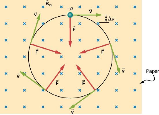
In this situation, the magnetic force supplies the centripetal force \(F_C = \dfrac{mv^2}{r}\). Noting that the velocity is perpendicular to the magnetic field, the magnitude of the magnetic force is reduced to \(F = qvB\).

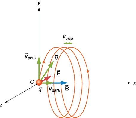
If the velocity is not perpendicular to the magnetic field, then we can compare each component of the velocity separately with the magnetic field. The component of the velocity perpendicular to the magnetic field produces a magnetic force perpendicular to both this velocity and the field:

\[\begin{align} v_{perp} &= v \, \sin \theta \\[4pt] v_{para} &= v \, \cos \theta. \end{align}\]

where \(\theta\) is the angle between v and B. The component parallel to the magnetic field creates constant motion along the same direction as the magnetic field, also shown in Equation. The parallel motion determines the pitch p of the helix, which is the distance between adjacent turns. This distance equals the parallel component of the velocity times the period:

\[p = v_{para} T. \label{11.8}\]

The result is a helical motion, as shown in the following figure.

Figure \(\PageIndex{2}\): A charged particle moving with a velocity not in the same direction as the magnetic field. The velocity component perpendicular to the magnetic field creates circular motion, whereas the component of the velocity parallel to the field moves the particle along a straight line. The pitch is the horizontal distance between two consecutive circles. The resulting motion is helical.

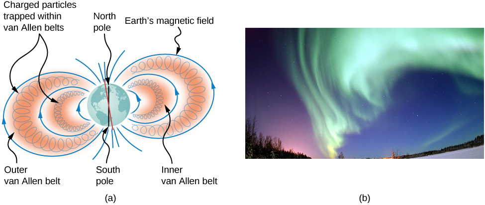
While the charged particle travels in a helical path, it may enter a region where the magnetic field is not uniform. In particular, suppose a particle travels from a region of strong magnetic field to a region of weaker field, then back to a region of stronger field. The particle may reflect back before entering the stronger magnetic field region. This is similar to a wave on a string traveling from a very light, thin string to a hard wall and reflecting backward. If the reflection happens at both ends, the particle is trapped in a so-called magnetic bottle.

Trapped particles in magnetic fields are found in the Van Allen radiation belts around Earth, which are part of Earth’s magnetic field. These belts were discovered by James Van Allen while trying to measure the flux of cosmic rays on Earth (high-energy particles that come from outside the solar system) to see whether this was similar to the flux measured on Earth. Van Allen found that due to the contribution of particles trapped in Earth’s magnetic field, the flux was much higher on Earth than in outer space. Aurorae, like the famous aurora borealis (northern lights) in the Northern Hemisphere (Figure \(\PageIndex{3}\)), are beautiful displays of light emitted as ions recombine with electrons entering the atmosphere as they spiral along magnetic field lines. (The ions are primarily oxygen and nitrogen atoms that are initially ionized by collisions with energetic particles in Earth’s atmosphere.) Aurorae have also been observed on other planets, such as Jupiter and Saturn.

Figure \(\PageIndex{3}\): (a) The Van Allen radiation belts around Earth trap ions produced by cosmic rays striking Earth’s atmosphere. (b) The magnificent spectacle of the aurora borealis, or northern lights, glows in the northern sky above Bear Lake near Eielson Air Force Base, Alaska. Shaped by Earth’s magnetic field, this light is produced by glowing molecules and ions of oxygen and nitrogen. (credit b: modification of work by USAF Senior Airman Joshua Strang)

Representing Magnetic Fields

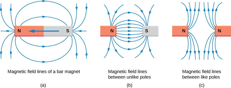
The representation of magnetic fields by magnetic field lines is very useful in visualizing the strength and direction of the magnetic field. As shown in Figure \(\PageIndex{3}\), each of these lines forms a closed loop, even if not shown by the constraints of the space available for the figure. The field lines emerge from the north pole (N), loop around to the south pole (S), and continue through the bar magnet back to the north pole.

Magnetic field lines have several hard-and-fast rules:

1. The direction of the magnetic field is tangent to the field line at any point in space. A small compass will point in the direction of the field line.
2. The strength of the field is proportional to the closeness of the lines. It is exactly proportional to the number of lines per unit area perpendicular to the lines (called the areal density).
3. Magnetic field lines can never cross, meaning that the field is unique at any point in space.
4. Magnetic field lines are continuous, forming closed loops without a beginning or end. They are directed from the north pole to the south pole.

The last property is related to the fact that the north and south poles cannot be separated. It is a distinct difference from electric field lines, which generally begin on positive charges and end on negative charges or at infinity. If isolated magnetic charges (referred to as magnetic monopoles) existed, then magnetic field lines would begin and end on them.

Figure \(\PageIndex{3}\): Magnetic field lines are defined to have the direction in which a small compass points when placed at a location in the field. The strength of the field is proportional to the closeness (or density) of the lines. If the interior of the magnet could be probed, the field lines would be found to form continuous, closed loops. To fit in a reasonable space, some of these drawings may not show the closing of the loops; however, if enough space were provided, the loops would be closed.

Contributors and Attributions

Samuel J. Ling (Truman State University), Jeff Sanny (Loyola Marymount University), and Bill Moebs with many contributing authors. This work is licensed by OpenStax University Physics under a Creative Commons Attribution License (by 4.0).