1.4: Electromagnetic Spectrum

Learning Objectives

By the end of this section, you will be able to:

• Define electromagnetic spectrum
• Identify ranges in the electromagnetic spectrum corresponding to different physical phenomena.
• Identify ranges in the radio-frequency spectrum and their applications.

Electromagnetic waves are oscillating disturbances in the electromagnetic field. The frequency of the wave is the number of oscillations per second and is given in units of Hertz (1 Hz = 1 oscillation per second). Electromagnetic fields exist at frequencies from 0 Hz to at least 10²⁰ Hz – that’s at least 20 orders of magnitude! At 0 Hz, electromagnetics consists of two distinct disciplines: electrostatics, concerned with electric fields, and magnetostatics, concerned with magnetic fields. At higher frequencies, electric and magnetic fields interact to form propagating waves. Waves having frequencies within certain ranges are given names based on how they manifest as physical phenomena. These names are (in order of increasing frequency) radio, infrared (IR), optical (also known as “light”), ultraviolet (UV), X-rays, and gamma rays (γ-rays). See Table \(\PageIndex{1}\) for the corresponding frequency ranges.

Definition: Electromagnetic Spectrum

The term electromagnetic spectrum refers to the various forms of electromagnetic phenomena that exist over the continuum of frequencies [1].

The speed (properly known as “phase velocity”) at which electromagnetic fields propagate in free space is given the symbol \(c\), and has the value of 299,792,458 m/s (exactly) or approximately \(3.00 \times 10^{8}\) m/s. This value is often referred to as the “speed of light.” While it is certainly the speed of light in free space, it is also the speed of any electromagnetic wave in free space. Given frequency \(f\), wavelength is given by the expression

\[ \underbrace{\lambda = \frac { c } { f }}_{\text{in free space}} \label{wavelength} \]

A sinusoidal wave repeats itself in space over a distance of the wavelength, as illustrated in Figure \(\PageIndex{1}\). According to Eq. \(\ref{wavelength}\), the wavelength and frequency are inversely related so that as one increases, the other decreases. To a good approximation, the wavelength in meters can then be calculated as 300 (in Mm) divided by the frequency in MHz.

Figure \(\PageIndex{1}\): Wavelength \(\lambda\) for a sinusoidal wave. [2]

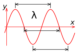
Table \(\PageIndex{1}\) shows the free space wavelengths associated with each of the regions of the electromagnetic spectrum.

Table \(\PageIndex{1}\): The electromagnetic spectrum. Note that the indicated ranges are arbitrary but consistent with common usage.

Regime	Frequency Range	Wavelength Range
\(\gamma\)-Ray	\(\mathrm{> 3 \times 10^{19} \; Hz}\)	< 0.01 nm
X-Ray	\(\mathrm{3 \times 10^{16} \; Hz \; – \; 3 \times 10^{19} \; Hz}\)	10–0.01 nm
Ultraviolet (UV)	\(\mathrm{2.5 \times 10^{15} \; – \; 3 \times 10^{16} \; Hz}\)	120–10 nm
Optical	\(\mathrm{4.3 \times 10^{14} \; – \; 2.5 \times 10^{15} \; Hz}\)	700–120 nm
Infrared (IR)	\(\mathrm{300 \; GHz \; – \; 4.3 \times 10^{14} \; Hz}\)	1 mm – 700 nm
Radio	\(\mathrm{3 \; kHz – 300 \; GHz}\)	100 km – 1 mm

This book presents a version of electromagnetic theory that is based on classical physics. This approach works well for most practical problems. However, at very high frequencies, wavelengths become small enough that quantum mechanical effects may be important. This effect usually happens in the X-ray band and above. In some applications, these effects become important at frequencies as low as the optical, IR, or radio bands. (A prime example is the photoelectric effect. [3]) Thus, caution is required when applying the classical version of the electromagnetic theory presented here, especially at these higher frequencies.

Caution

The theory presented in this book applies to static fields (0 Hz) along with radio, infrared, and light waves and, to a lesser extent, to ultraviolet waves, X-rays, and gamma rays. Certain phenomena in these frequency ranges – in particular, quantum mechanical effects – are not addressed in this book.

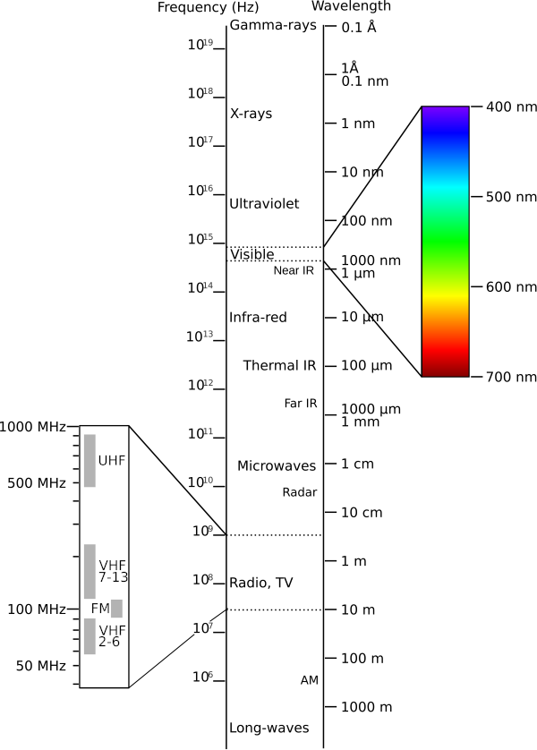
The radio-frequency (RF) portion of the electromagnetic spectrum alone spans 12 orders of magnitude in frequency (and wavelength), and so, not surprisingly, exhibits a broad range of phenomena (Figure \(\PageIndex{2}\)). For this reason, the radio spectrum is further subdivided into bands as shown in Table \(\PageIndex{2}\) [4]. Also shown in Table \(\PageIndex{2}\) are commonly used band identification acronyms and some typical applications. Amateur Radio operators can use portions of the radio bands starting as low as the Low Frequency (LF) band through the Extremely High Frequency (EHF) band and beyond, depending on their license class. However, in practice, activity for Amateur Radio tends to occur primarily on the High Frequency (HF), Very High Frequency (VHF), and Ultra High Frequency (UHF) bands.

Similarly, the optical band is partitioned into the familiar "rainbow" of red through violet, as shown in Figure \(\PageIndex{2}\) and Table \(\PageIndex{3}\). Other portions of the spectrum are sometimes similarly subdivided in certain applications.

Figure \(\PageIndex{2}\): Electromagnetic Spectrum.

Table \(\PageIndex{2}\): The radio-frequency (RF) portion of the electromagnetic spectrum, according to a common scheme for naming ranges of radio frequencies from the International Telecommunication Union. WLAN: Wireless local area network, LMR: Land mobile radio, RFID: Radio frequency identification [5].

Band	Frequencies	Wavelengths	Typical Applications
THF (Tremendously High Frequency)	300–3000 GHz (0.3–3 THz)	1–0.1 mm	Short-range communication, Imaging, Spectroscopy
EHF (Extremely High Frequency)	30–300 GHz	10–1 mm	60 GHz WLAN, Point-to-point data links
SHF (Super High Frequency)	3–30 GHz	10–1 cm	Terrestrial & Satellite data links, Radar
UHF (Ultra High Frequency)	300–3000 MHz	1–0.1 m	TV broadcasting, Cellular, WLAN
VHF (Very High Frequency)	30–300 MHz	10–1 m	FM & TV broadcasting, LMR
HF (High Frequency)	3–30 MHz	100–10 m	Global terrestrial comm., CB Radio
MF (Medium Frequency)	300–3000 kHz	1000–100 m	AM broadcasting
LF (Low Frequency)	30–300 kHz	10–1 km	Navigation, RFID
VLF (Very Low Frequency)	3–30 kHz	100–10 km	Navigation
ULF (Ultra Low Frequency)	300–3000 Hz	1000–100 km	Underground communication
SLF (Super Low Frequency)	30–300 Hz	10000–1000 km	Underwater communication
ELF (Extremely Low Frequency)	3–30 Hz	100000–10000 km	Underwater communication, Lightning

Table \(\PageIndex{3}\): The optical portion of the electromagnetic spectrum.

Band	Frequencies	Wavelengths
Violet	668–789 THz	450–380 nm
Blue	606–668 THz	495–450 nm
Green	526–606 THz	570–495 nm
Yellow	508–526 THz	590–570 nm
Orange	484–508 THz	620–590 nm
Red	400–484 THz	750–620 nm

References

1. Wikipedia contributors. Electromagnetic spectrum [Internet]. Wikipedia, The Free Encyclopedia.
2. Wikimedia Commons contributors. File:Sine wavelength.svg [Internet]. Wikimedia Commons. (CC BY-SA 3.0, Richard F. Lyon)
3. Wikipedia contributors. Photoelectric effect [Internet]. Wikipedia, The Free Encyclopedia.
4. Wikipedia contributors. Radio spectrum [Internet]. Wikipedia, The Free Encyclopedia.
5. Wikimedia Commons contributors. File:Electromagnetic-Spectrum.svg [Internet]. Wikimedia Commons. (CC BY-SA 3.0, V. Blacus)

Technician Exam Questions

The Radio Spectrum

Relevant exam questions include: T3B08‒10, T5A06, T5A12, T5C06.

Wavelength

Relevant exam questions include: T3B04‒07, T3B11.