2.4: Electric Fields and Forces

LEARNING OBJECTIVES

By the end of this section, you will be able to:

• Explain the purpose of the electric field concept
• Describe the properties of the electric field
• Calculate the electric force that charges exert on each other
• Determine the direction of the electric force for different source charges

Having seen the qualitative effects of charged objects on other charged objects, we would also like to be able to calculate quantities related to these effects. In this section, we will begin to define our approach to these calculations.

Defining a Field

We have seen experimentally that electric charges can have effects over a distance without contact. It is then natural to hypothesize that a physical field around a charged particle exists that can exert force on other charged particles. Mathematically, a physical field is a function that gives a value of a physical quantity at each point in space and each moment in time (see Example \(\PageIndex{1}\) and Example \(\PageIndex{2}\)).

Example \(\PageIndex{1}\)

In weather reports, a temperature field can be visualized on a map showing the temperature's value at each point on the map at a specific moment in time. Because each temperature is a number, this field is known as a scalar field.

Figure \(\PageIndex{1}\): Temperature field visualized in a map format. In the image, the values of temperature are given in degrees Celsius and are also color-coded. From the map, you can see that it is warmest in the southwestern states and coolest in the northern states and western mountainous regions. [1]

Example \(\PageIndex{2}\)

Weather reports will also sometimes give a wind velocity field. In this case, the map shows the magnitude and direction of the wind at each point on the map at a specific moment in time. Because the wind velocity is a vector, this field is known as a vector field.

Figure \(\PageIndex{2}\): Wind velocity field visualized in a map format. In this map, the wind direction is given by wind barbs that point to the direction from which the wind is coming, while the speed is given by the color coding in kilometers per hour (1 kph = 1 km/h). The map shows it is windiest in the north-central United States and the Atlantic Ocean off of the East Coast. [2]

Defining the Electric Field

Because we expect the field around a charge to exert a force, which is a vector quantity, we will hypothesize that the electric field is a vector field. For simplicity, we will start by considering the source of the field to be a single point charge, which we define as an idealized particle at a single point in space at coordinates \( (x_s, y_s, z_s) \) carrying a specified source charge \( q \). Based on experimental evidence, we define the electric field at test location \( (x_t, y_t, z_t) \) away from the source charge to be

\[\vec{E} = \dfrac{1}{4 \pi \epsilon_0} \dfrac{q}{r^2}\hat{r}, \label{Efield0} \]

where \(\epsilon_0\) is the permittivity of free space (vacuum), \( r \) is the separation distance between the source charge and test location, and \( \hat{r} \) is the radial unit vector that points in the direction from the source charge to the test location. From geometry, the distance between the source charge and test location is given by

\[ r = [(\Delta x)^2 + (\Delta y)^2 + (\Delta z)^2]^{1/2}, \label{rdistance} \]

where \( \Delta x = x_t - x_s \), \( \Delta y = y_t - t=y_s \), \( \Delta z = z_t - z_s \) are the differences in coordinates between the test and source charges. Note that the Also, from geometry, the radial unit vector is

\[ \hat{r} = \dfrac{(\Delta x)\hat{i}+(\Delta y)\hat{j}+(\Delta z)\hat{k}}{[(\Delta x)^2 + (\Delta y)^2 + (\Delta z)^2]^{1/2}} \label{rhat} \]

The radial unit vector in Equation \ref{Efield0} ensures that the electric field is always directed along the line between the source charge and the test location. The numerator sets the proper direction, while the denominator ensures that the length of the unit vector is one.

Direction of the Radial Unit Vector

The radial unit vector always points away from the source charge and toward the test location. You can remember this relation from the "rst" memory aid:

r-hat points from
source to
test

This is true regardless of the sign of the source charge, as Equation \ref{rhat} does not contain any charge terms.

A consequence of Equation \ref{Efield0} is that the direction of the electric field is determined by the sign of the source charge. If the source charge is positive, the electric field points in the same direction as the radial unit vector (outward). If the source charge is negative, the electric field points in the opposite direction as the radial unit vector (inward).

Direction of the Electric Field

By convention, all electric fields \(\vec{E}\) point away from positive source charges and point toward negative source charges.

It is important to emphasize that the electric field is not constant around a point charge but instead falls off as the reciprocal of the square of the separation distance. In addition, if either the source charge's location or the test location moves, then \( r \) and \(\hat{r}\) change, and therefore, so does the electric field.

The permittivity of free space has a very important physical meaning that we will discuss in a later chapter; for now, it is simply an empirical proportionality constant. Its numerical value (to three significant figures) turns out to be

\[\epsilon_0 = 8.85 \times 10^{-12} \dfrac{\mathrm{C}^2}{\mathrm{N} \cdot \mathrm{m}^2}.\]

These units are required to give the electric field in the correct units of newtons per coulomb. For convenience, we often define the electrostatic constant (also known as Coulomb's constant) to be

\[ k = \dfrac{1}{4\pi \epsilon_0} = 8.99 \times 10^9 \dfrac{\mathrm{N} \cdot \mathrm{m}^2}{\mathrm{C}^2}.\]

A consequence of these constants being given in units of meters and coulombs is that the charge and separation distance in Equation \ref{Efield0} must also be given those same units to ensure that the force is in units of newtons.

Strictly speaking, Equation \ref{Efield0} is only valid for a point charge. However, it will still usually be a good approximation for the electric field of a uniformly charged particle at distances that are large compared to the size of the particle. Example \(\PageIndex{3}\) shows how you can calculate electric fields and forces for a problem with two point charges.

Example \(\PageIndex{3}\)

Electric Field Due to Point Charges

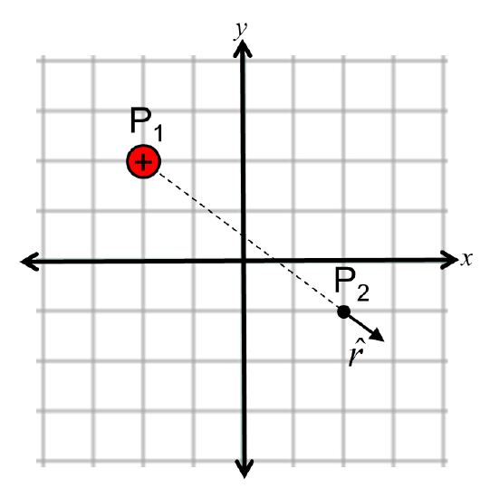
(a) Suppose a point charge of +5.00nC is located at Point \( P_1 \) with coordinates \( (-2.00\ \mathrm{m}, +2.00\ \mathrm{m}, 0.00\ \mathrm{m}) \). What is the electric field at Point \( P_2 \) \( (+2.00\ \mathrm{m}, +1.00\ \mathrm{m}, 0.00\ \mathrm{m}) \)?

(b) What is the strength (magnitude) of the electric field at \( (+2.00\ \mathrm{m}, +1.00\ \mathrm{m}, 0.00\ \mathrm{m}) \)?

Solution

(a) We will follow a four-step problem-solving strategy:

PLAN We have a point charge, so we plan to use Eq. \(\ref{Efield0}\) to find the electric field.

SKETCH However, before we start to calculate, it is important to make a drawing of the geometry of the problem, marking the source charge at Point \( P_1 \) and the test location at Point \( P_2 \). We can also sketch in the direction of the radial unit vector because we know it lines along the line connecting Points \( P_1 \) and \( P_2 \) and points away from the source charge and toward the test location. We will later use the sketch to check our calculations.

Figure \(\PageIndex{3}\): Sketch of the source charge and test location for part (a) of Example \(\PageIndex{3}\). [4]

CALCULATE To use Eq. \(\ref{Efield0}\), we must first know the charge, separation distance, and radial unit vector. We first convert the charge to coulombs by writing \( q = 5\ \mathrm{nC} = 5 \times 10^{-9}\ \mathrm{C}\). Next, we identify the location of the source charge as \( (x_s, y_s, z_s) = (-2.00\ \mathrm{m}, +2.00\ \mathrm{m}, 0.00\ \mathrm{m}) \) and the test location as \( (x_t, y_t, z_t) = (+2.00\ \mathrm{m}, -1.00\ \mathrm{m}, 0.00\ \mathrm{m}) \). As a result,

\[ \begin{align*}
\Delta x &= x_t - x_s = +2.00\ \mathrm{m} - -2.00\ \mathrm{m} = +4.00\ \mathrm{m},\\
\Delta y &= y_t - y_s = -1.00\ \mathrm{m} - 2.00\ \mathrm{m} = -3.00\ \mathrm{m}, \\
\Delta z & = z_t - z_s = 0.00\ \mathrm{m} - 0.00\ \mathrm{m} = 0.00\ \mathrm{m},
\end{align*} \]

and therefore the separation distance is given by Equation \ref{rdistance}

\[ r = [(\Delta x)^2 + (\Delta y)^2 + (\Delta z)^2]^{1/2} = [(+4.00\ \mathrm{m})^2 + (-3.00\ \mathrm{m})^2 + (0.00\ \mathrm{m})^2]^{1/2} = 5.00\ \mathrm{m}. \nonumber \]

The radial unit vector is then given by Equation \ref{rhat}

\[ \hat{r} = \dfrac{(\Delta x)\hat{i}+(\Delta y)\hat{j}+(\Delta z)\hat{k}}{[(\Delta x)^2 + (\Delta y)^2 + (\Delta z)^2]^{1/2}}
= \dfrac{(+4.00\ \mathrm{m})\hat{i}+(-3.00\ \mathrm{m})\hat{j}+(0.00\ \mathrm{m})\hat{k}}{5.00\ \mathrm{m}}
= +0.800 \hat{i} - 0.600\hat{j}.
\nonumber \]

Observe that the radial unit vector is always dimensionless; the dimensions come from the other quantities in the problem. The electric field at the test location is then given by Eq. \(\ref{Efield0}\)

\[ \vec{E} = \dfrac{1}{4 \pi \epsilon_0} \dfrac{q}{r^2}\hat{r}
= \left(8.99 \times 10^9 \dfrac{\mathrm{N} \cdot \mathrm{m}^2}{\mathrm{C}^2}\right)
\dfrac{5.00 \times 10^{-9}\ \mathrm{C}}{(5.00\ \mathrm{m})^2}(0.800 \hat{i} - 0.600\hat{j})
=(+1.44\ \mathrm{N/C})\hat{i} +(-1.08\ \mathrm{N/C})\hat{j}
\]

CHECK The calculated electric field vector indicates that the vector points down and to the right, a result which is consistent with Fig. \(\PageIndex{3}\). It also indicates that the x-component is larger than the y-component, which is also consistent with the diagram. Finally, the units are in newtons per coulomb, as expected.

(b) The strength of the electric field is the magnitude of the electric field vector

\[|\vec{E}| = \dfrac{1}{4 \pi \epsilon_0} \dfrac{|q|}{r^2}=[(+1.44\ \mathrm{N/C})^2+(-1.08\ \mathrm{N/C})^2]^{1/2} = 1.80\ \mathrm{N/C}\]

Defining Electric Force

Experiments with electric charges have shown that if two objects each have electric charge, then they exert an electric force on each other. The electric field is useful because once we know the electric field at a test location, we can then calculate the electric force \(\vec{F}\) on a point charge \( Q \) ("test charge") placed at that test location simply by multiplying the charge and electric field together

\[\vec{F_E} = Q \vec{E}. \label{Efield1} \]

With charge in coulombs (C) and electric field in newtons per coulombs (N/C) , their product will be in newtons, as expected for force. Example \(\PageIndex{4}\) show how you can calculate electric force between two point charges.

Example \(\PageIndex{4}\)

Continuing with the scenario of Example \( \PageIndex{3}\),

(a) Suppose a second point charge of −3.00 nC is now placed at Point \( P_2 \). What is the electric force exerted on this new second charge of −3.00 nC due to the original charge of +5.00 nC?

(b) What is the electric force exerted on the original charge of +5.00 nC due to the second charge of −3.00 nC?

Solution

(a) We will follow a four-step problem-solving strategy:

PLAN Because we already know the electric field at Point \( P_2 \) and are given a second point charge, we can use Equation \ref{Efield1} to find the electric force.

SKETCH We can modify our previous diagram to show the geometry of both charges relative to each other. It is also a good idea to draw the radial unit vector and vectors in the expected directions of the electric field and electric force. Note that the radial unit vector still points in the same direction as in Fig. \(\PageIndex{3}\) because the +5 nC charge is still the source charge creating the electric field that is exerting the electric force on the −3 nC charge. The electric field vector is in the same direction as the radial unit vector because the source charge is positive. However, the direction of the electric force is in the opposite direction of the radial unit vector because we know that positive and negative charges attract.

Figure \(\PageIndex{4}\): Sketch of charges, radial unit vector, electric field vector, and electric force vector for part (a) of Example \(\PageIndex{4}\). [4]

CALCULATE The electric force is given by Equation \ref{Efield1}

\[ \vec{F_E} = Q \vec{E} = (-3.00\times 10^{-9}\ \mathrm{C})[(+1.44\ \mathrm{N/C})\hat{i} +(-1.08\ \mathrm{N/C})\hat{j}]
= (-4.31\times 10^{-7}\ \mathrm{N})\hat{i} +(3.24\times 10^{-7}\ \mathrm{N})\hat{j} \nonumber \]

Note that the test charge must be written in coulombs in Equation \ref{Efield1} to ensure the force is in newtons.

CHECK The calculated force is directed left and up, a result which is consistent with the expected attractive force.

(b) In this question, we are asked to find the electric force exerted by the second charge of −3.00 nC on the +5.00 nC charge. In other words, the charges have switched roles, so the −3.00 nC charge is now the source charge and the +5.00 nC charge is the test charge. The electric field at Point \( P_1 \) due to the −3.00 nC charge can then be calculated using the same approach as in Example \(\PageIndex{3}\).

The location of the source charge is \( (x_s, y_s, z_s) = (+2.00\ \mathrm{m}, -1.00\ \mathrm{m}, 0.00\ \mathrm{m}) \), while the test location is \( (x_t, y_t, z_t) = (-2.00\ \mathrm{m}, +2.00\ \mathrm{m}, 0.00\ \mathrm{m}) \). As a result,

\[ \begin{align*}
\Delta x &= x_t - x_s = -2.00\ \mathrm{m} - 2.00\ \mathrm{m} = -4.00\ \mathrm{m},\\
\Delta y &= y_t - y_s = 2.00\ \mathrm{m} - -1.00\ \mathrm{m} = +3.00\ \mathrm{m}, \\
\Delta z & = z_t - z_s = 0.00\ \mathrm{m} - 0.00\ \mathrm{m} = 0.00\ \mathrm{m},
\end{align*} \]

and therefore the separation distance is given by Equation \ref{rdistance}

\[ r = [(\Delta x)^2 + (\Delta y)^2 + (\Delta z)^2]^{1/2} = [(-4.00\ \mathrm{m})^2 + (+3.00\ \mathrm{m})^2 + (0.00\ \mathrm{m})^2]^{1/2} = 5.00\ \mathrm{m}. \nonumber \]

The radial unit vector is then given by Equation \ref{rhat}

\[ \hat{r} = \dfrac{(\Delta x)\hat{i}+(\Delta y)\hat{j}+(\Delta z)\hat{k}}{[(\Delta x)^2 + (\Delta y)^2 + (\Delta z)^2]^{1/2}}
= \dfrac{(-4.00\ \mathrm{m})\hat{i}+(3.00\ \mathrm+{m})\hat{j}+(0.00\ \mathrm{m})\hat{k}}{5.00\ \mathrm{m}}
= -0.800 \hat{i} + 0.600\hat{j}.
\nonumber \]

The electric field at the test location of Point \( P_1 \) is given by Eq. \(\ref{Efield0}\)

\[ \vec{E} = \dfrac{1}{4 \pi \epsilon_0} \dfrac{q}{r^2}\hat{r}
= \left(8.99 \times 10^9 \dfrac{\mathrm{N} \cdot \mathrm{m}^2}{\mathrm{C}^2}\right)
\dfrac{-3.00 \times 10^{-9}\ \mathrm{C}}{(5.00\ \mathrm{m})^2}(-0.800 \hat{i} + 0.600\hat{j})
=(+0.863\ \mathrm{N/C})\hat{i} +(-0.647\ \mathrm{N/C})\hat{j}
\nonumber \]

According to Equation \ref{Efield1}, the electric force on the +5 nC charge is then

\[ \vec{F_E} = Q \vec{E} = (+5.00\times 10^{-9}\ \mathrm{C})[(0.863\ \mathrm{N/C})\hat{i} +(-0.647\ \mathrm{N/C})\hat{j}]
= (+4.31\times 10^{-7}\ \mathrm{N})\hat{i} + (-3.24\times 10^{-7}\ \mathrm{N})\hat{j} \nonumber \]

We see that the force has the same magnitude as in part (a) but opposite direction. This result should be expected because we know from experiments that the positive and negative charges attract.

PhET Simulation: Electric Field of Dreams

Open the Electric Field of Dreams applet.  This applet allows you to construct an electric field and then insert one or more charged particles into the field.

Instructions:

1. Open the applet and choose the appropriate emulation for your system (usually CheepJ will work).  
2. Click on the blue dot in the "External Field" box and then drag it in some direction to define the magnitude and direction of the electric field.
3. Press the Click on the "Properties" button, and then enter the desired values of charge and mass for a particle.
4. Click on the "Add" button to add the particle to the field.  Is the motion of the particle make sense?  Is it consistent with Eq. (\(\PageIndex{8}\))?
5. Click on the "Properties" button again, and change the properties to have the opposite sign of charge.  Click on the "Add" button to add this second particle. 
6. Observe the motion of the particles together.  Does the motion of the second particle make sense?  Can you see the particles interacting with each other?

Source: Electric Field of Dreams

Simulation by PhET Interactive Simulations, University of Colorado Boulder, licensed under CC-BY-4.0 (opens in new window).

Coulomb's Law

Substituting Equation \ref{Efield0} into Equation \ref{Efield1} yields an equation that allows you to calculate the electric force between two point charges directly. This equation is usually called Coulomb's Law.

Coulomb's Law

The electric force exerted by a point charge \( q_1 \) on a point charge \( q_2 \) separated by a distance \( r_{12} \) is equal to

\[ \vec{F}_{12} = \dfrac{1}{4 \pi \epsilon_0} \dfrac{q_{1} q_{2}}{r_{12}^2}\hat{r}_{12}, \label{Coulomb} \]

where \(\hat{r}_{12}\) is the radial unit vector directed from the location of charge \( q_1 \) to the location of charge \( q_2 \).

We see that the magnitude of electric force is proportional to the product of the charges and inversely proportional to the square of the separation distance between the charges. The form of Equation \ref{Coulomb} shows more clearly why the electric forces calculated in parts (a) and (b) in Example \(\PageIndex{4}\) must be equal in magnitude, because the magnitude of the force does not change if the roles of \( q_1 \) and \( q_2 \) are reversed and must be opposite in direction because \( \hat{r}_{12} = -\hat{r}_{21} \).

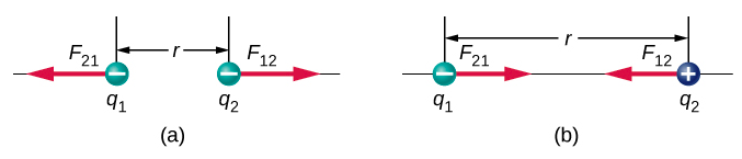
Observe that Coulomb's Law allows the electric forces between two charges to be repulsive or attractive. If the charges have the same sign, then their product is positive, the electric force is in the same direction as \(\hat{r}\), and the force is repulsive. If the charges have opposite signs, then their product is negative, the force is in the opposite direction of \(\hat{r}\), and the force is attractive. This idea is illustrated in Figure \(\PageIndex{5}\).

Figure \(\PageIndex{5}\): The electrostatic force \(\vec{F}\) between point charges \(q_1\) and \(q_2\) separated by a distance \(r\) is given by Coulomb’s law. Note that Newton’s third law (every force exerted creates an equal and opposite force) applies as usual—the force on \(q_1\) is equal in magnitude and opposite in direction to the force it exerts on \(q_2\). (a) Like charges; (b) unlike charges.

The following interactive simulation further illustrates the qualitative and quantitative properties of Coulomb's Law.

PhET Simulation: Coulomb's Law

Instructions:

1. Select "Macro Scale".
2. Move the slider back and forth for Charge 1 to adjust its charge from negative to zero to positive. How do the forces on the charges change?
3. Move the slider back and forth for Charge 2 to adjust its charge from negative to zero to positive. How do the forces on the charges change?
4. Is there a scenario where the forces are ever unequal in magnitude or in the same direction?
5. Move Charge 1 to the zero position, and then move the position of Charge 2. Does the inverse square law hold?
6. Bonus: Select the "Atomic Scale" button at the bottom of the screen. How do the results change at the smaller scale?
   
   

Source: Coulomb's Law

Simulation by PhET Interactive Simulations, University of Colorado Boulder, licensed under CC-BY-4.0 (opens in new window).

Example \(\PageIndex{5}\) shows how Coulomb's Law can be applied to a familiar system of two charges, the hydrogen atom.

Example \(\PageIndex{5}\): The Force on the Electron in Hydrogen

A hydrogen atom consists of a single proton and a single electron. The proton has a charge of \(+e\), and the electron has \(-e\). In the “ground state” of the atom, the electron orbits the proton at the most probable distance of \(5.29 \times 10^{-11}\ \mathrm{m}\) ). Calculate the electric force on the electron due to the proton.

PLAN  For the purposes of this example, we are treating the electron and proton as two point particles, each with an electric charge, and we are told the distance between them; we are asked to calculate the force on the electron. We thus use Coulomb’s law (Equation \ref{Coulomb}).

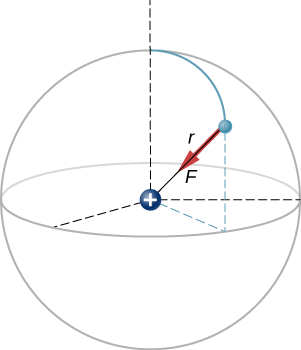
SKETCH  Figure \(\PageIndex{6}\) shows a diagram the hydrogen atom with the force vector marked.

Figure \(\PageIndex{6}\): A schematic depiction of a hydrogen atom, showing the force on the electron. This depiction is only to enable us to calculate the force; the hydrogen atom does not really look like this.

CALCULATE  Our two charges are \( q_1 = +e = +1.602 \times 10^{-19}\ \mathrm{C}\) and \( q_2 = -e = -1.602 \times 10^{-19}\ \mathrm{C} \), and the distance between them is given to be \(r = 5.29 \times 10^{-11}\ \mathrm{m}\).

The force on the electron from Equation \ref{Coulomb} is

\[\begin{align*}
\vec{F_E} &= \dfrac{1}{4\pi \epsilon_0}\dfrac{q_1 q_2}{r_{12}^2} \hat{r}\\[4pt]
&= \dfrac{1}{4\pi \left(8.85 \times 10^{-12} \frac{\mathrm{C}^2}{\mathrm{N} \cdot \mathrm{m}^2} \right)} \dfrac{(1.602 \times 10^{-19}\ \mathrm{C})(-1.602 \times 10^{-19}\ \mathrm{C})}{(5.29 \times 10^{-11}\ \mathrm{m})^2} \\[4pt]
&= (8.25 \times 10^{-8}\ \mathrm{N})(-\hat{r})
\end{align*}\]

Because the charges on the two particles are opposite, the force is negative (attractive); the force on the electron points radially directly toward the proton, everywhere in the electron’s orbit.

CHECK  This is a three-dimensional system, so the electron (and therefore the force on it) can be anywhere in an imaginary spherical shell around the proton. In this “classical” model of the hydrogen atom, the electrostatic force on the electron points in the inward centripetal direction, thus maintaining the electron’s orbit. However, the more accurate quantum-mechanical model of hydrogen (discussed in Quantum Mechanics) is utterly different.

If you have studied Newtonian mechanics, you will be familiar with gravitational fields as another type of fundamental physical field. Interestingly, there are parallels between electric and gravitational fields and forces, as discussed in Example \(\PageIndex{6}\).

Example \(\PageIndex{6}\)

Comparison: Gravitational Fields & Forces vs. Electric Fields & Forces

The mathematical equation for the electric field \(\vec{E}\) of a point charge (Equation \ref{Efield0}) is similar to the gravitational field \(\vec{g}\) of Earth

\[\vec{g} = -G \dfrac{M_e}{r^2}\hat{r}, \label{gfield0} \]

where \( G = 6.67 \times 10^{-11}\ \mathrm{N}\cdot\mathrm{m}^2/\mathrm{kg}^2 \) is the gravitational constant, \( M_e = 5.98\times 10^{24}\ \mathrm{kg}\) is the mass of the Earth, and \( r \) is the distance away from the Earth's center, assuming the Earth is approximately spherical. You can see that the proportionality constant \(G\) plays the same role for the gravitational field \(\vec{g}\) as the electrostatic constant \(k = \frac{1}{4\pi \epsilon_0}\) does for the electric field \(\vec{E}\).

On the surface of the Earth, the distance \( r = R_e = 6.37 \times 10^6\ \mathrm{m}\) is the radius of the Earth, and Equation \ref{gfield0} reduces down to

\[\vec{g} = -G\dfrac{M_e}{R_e^2}\hat{r} = (9.81\ \mathrm{N/kg})(-\hat{r}) \ \ \ \text{(On Earth's surface only)} \nonumber \]

The factor \( 9.81\ \mathrm{N/kg}= 9.81 \mathrm{m}/\mathrm{s}^2\) is recognized as the acceleration of gravity, and the factor \(-\hat{r}\) indicates that the force is attractive and directed toward the center of the Earth, as expected.

Once we have calculated the gravitational field at some point in space due to a source mass, we can use it any time we want to calculate the resulting force on any test mass we choose to place at that test location according to

\[\vec{F_G} = M \vec{g} . \label{gfield1} \]

In fact, this is exactly what we do when we calculate the force on different masses due to gravity (i.e., weight). You can see this equation is similar in form to Equation \ref{Efield1} for the electric force, with charge replacing mass. Combining Eqs. \ref{gfield0} and \ref{gfield1} yields the equation

\[ \vec{F}_{12} = -G \dfrac{m_{1} m_{2}}{r_{12}^2} \hat{r}_{12}, \label{NewtonGravity} \]

which is Newton's Law of Universal Gravitation and, similar to Coulomb's Law, is an inverse-square law in the separation distance.

One significant difference between Coulomb's Law and Newton's Law of Universal Gravitation is that charge can be positive or negative, whereas mass is only positive. As a result, gravity is always an attractive force, whereas electric forces can be attractive or repulsive.

The Meaning of "Electric Field"

Like the gravitational field of an object with mass, you should picture the electric field of a charge-bearing object (the source charge) as a continuous, immaterial substance that surrounds the source charge, filling all of space—in principle, to \(\pm \infty\) in all directions. The field exists at every physical point in space. To put it another way, the electric charge on an object alters the space around the charged object in such a way that all other electrically charged objects in space experience an electric force as a result of being in that field. The electric field, then, is the mechanism by which the electric properties of the source charge are transmitted to and through the rest of the universe. (Again, the range of the electric force is infinite.) We will see in subsequent chapters that the speed at which electrical phenomena travel is the same as the speed of light. There is a deep connection between the electric field and light.

In the next section, we describe how to determine the electric field and forces due to multiple individual source charges.

References

1. National Weather Service [Internet]. Graphical forecasts. 2024. National Weather Service. (Select "Temperature" and set the units to Celsius.) (Public domain)
2. National Weather Service [Internet]. Graphical forecasts. 2024. National Weather Service. (Select "Wind Speed".) (Public domain)
3. Wikipedia contributors. Euclidean distance [Internet]. Wikipedia, The Free Encyclopedia.
4. Wikimedia Commons contributors. File:Graph-paper.svg [Internet]. Wikimedia Commons. (CC-SA 3.0, Bobarino). Additional elements by Ronald Kumon (CC-BY-SA 4.0, Ronald Kumon).