3.7: Common Models of Electric Potential

Learning Objectives

By the end of this section, you will be able to:

• List and apply common models for the electric potential of continuous charge distributions.

Continuous Charge Distributions

As we saw previously in Common Models of Electric Field, there are situations where there are so many charges that the system can be modeled as a continuous distribution of charges. In other words, the superposition of electric potential as a sum of discrete contributions

\[V_p = k\sum \dfrac{q_i}{r_i}.\]

can be modeled instead as a continuous charge distribution consisting of a collection of infinitesimally separated individual points. This approach yields the integral

\[V_p = \int \dfrac{dq}{r}\]

for the potential at a point \(P\). Note that \(r\) is the distance from each individual point in the charge distribution to the point \(P\). As before, the infinitesimal charges are given by

\[\underbrace{dq = \lambda \, dl}_{\text{one dimension}}\]

\[\underbrace{dq = \sigma \, dA}_{\text{two dimensions}}\]

where \(\lambda\) is linear charge density and \(\sigma\) is the charge per unit area.

In this chapter, we will summarize several models corresponding to the most common geometric distributions of charge. In each of these models, the electric potential can be written in a closed-form expression for a specified region of space around the charge distribution. Students who are interested in the details of the calculations should refer to the section Calculating Electric Potentials of Charge Distributions in the chapter Direct Calculation of Electrical Quantities from Charge Distributions.

Electric Potentials of Common Charge Distributions

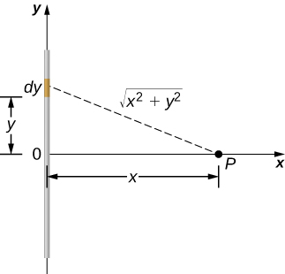
Finite Line Segment of Charge

Suppose a finite line segment of charge is located along the y-axis as illustrated in Fig. \(\PageIndex{1}\). Assume that the segment has charge density \(\lambda\) (e.g., in coulombs per meters). The electric potential along the perpendicular bisector of the segment at a distance \(x\) away from the segment is

\[ V(x) = k\lambda \ln \left[ \dfrac{L + \sqrt{L^2 + 4x^2}}{-L + \sqrt{L^2 + 4x^2}}\right] \label{Vlinesegment}\].

Figure \(\PageIndex{1}\): Geometry for calculating electric potential due to a finite line of uniform charge density.

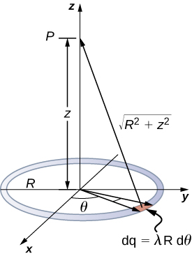
Ring of Charge

If we take a finite line segment with linear charge density \(\lambda\) and total charge \( q_0 \) and wrap it into a closed circular loop, then we get a ring of charge of radius \( R \) (Fig. \(\PageIndex{2}\)). The electric field at a distance \( z \) from the plane of the ring along its symmetry axis is

\[ V(z) = \dfrac{2\pi k \lambda R}{\sqrt{z^2 + R^2}} = k \dfrac{q_{tot}}{\sqrt{z^2 + R^2}} \label{Vring}\]

Figure \(\PageIndex{2}\): Geometry for calculating electric potential due to a ring of uniform charge density.

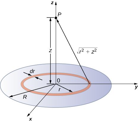
Disk of Charge

Once we know the electric field along the axis of a ring of charge, we can use this result to find the electric field along the axis of a disk of charge because a disk of charge can be modeled as a set of rings of charge of increasing radius (Fig. \(\PageIndex{3}\). The electric field for a disk of radius \(R\) and uniform surface charge density \(\sigma\) (coulombs per m\(^2\)) along the axis of the disk at a distance \(z\) from the disk is

\[ V(z) = k2\pi \sigma ( \sqrt{z^2 + R^2} - \sqrt{z^2}) \label{Vdisk} \]

Figure \(\PageIndex{3}\): Geometry for calculating the electric potential due to a disk of uniform surface charge density.

Infinite Line of Charge

Consider an infinite line of charge with linear charge density \(\lambda\) aligned along the \(y\)-axis. Assume the reference potential \(V_R = 0\ \textrm{V}\) at \(x = 1\ \textrm{m}\) from the line of charge. The electric potential at a distance \(x\) in meters perpendicular to the line is

\[ V(x) = -2 k\lambda \ln x. \label{Vinfiniteline} \]

Note that unlike the result for the finite line segment Equation \ref{Vlinesegment} where the reference potential for zero voltage was taken at infinity, here the reference voltage was taken at a finite distance of 1 meter from the wire. This specification is necessary because the charge itself reaches to infinity, and therefore the potential cannot be set to zero there.

Even though no actual infinite line charge exists, the result of Equation \ref{Vinfiniteline} can still provide a simple and good approximation for the potential provided that the separation distance to the test location is small compared to the length of the line charge.