16.4: Calculating Electric Potential of Charge Distributions

Learning Objectives

By the end of this section, you will be able to:

• Calculate the potential of various continuous charge distributions

How do you calculate the electric potential of continuous charge distributions? Recall that for multiple point charges,

\[V_p = k\sum \dfrac{q_i}{r_i}.\]

We may treat a continuous charge distribution as a collection of infinitesimally separated individual points. This yields the integral

\[V_p = \int \dfrac{dq}{r}\]

for the potential at a point \(P\). Note that \(r\) is the distance from each individual point in the charge distribution to the point \(P\). As we saw in Electric Charges and Fields, the infinitesimal charges are given by

\[\underbrace{dq = \lambda \, dl}_{\text{one dimension}}\]

\[\underbrace{dq = \sigma \, dA}_{\text{two dimensions}}\]

\[\underbrace{dq = \rho \, dV \space}_{\text{three dimensions}}\]

where \(\lambda\) is linear charge density, \(\sigma\) is the charge per unit area, and \(\rho\) is the charge per unit volume.

Example \(\PageIndex{1}\): Potential of a Line of Charge

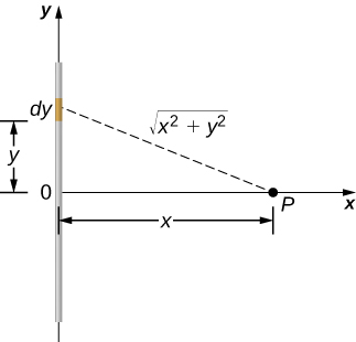
Find the electric potential of a uniformly charged, nonconducting wire with linear density \(\lambda\) (coulomb/meter) and length \(L\) at a point that lies on a line that divides the wire into two equal parts.

Strategy

To set up the problem, we choose Cartesian coordinates in such a way as to exploit the symmetry in the problem as much as possible. We place the origin at the center of the wire and orient the \(y\)-axis along the wire so that the ends of the wire are at \(y = \pm L/2\). The field point \(P\) is in the \(xy\)-plane and since the choice of axes is up to us, we choose the \(x\)-axis to pass through the field point \(P\), as shown in Figure \(\PageIndex{1}\).

Figure \(\PageIndex{1}\): We want to calculate the electric potential due to a line of charge.

Solution

Consider a small element of the charge distribution between \(y\) and \(y + dy\). The charge in this cell is \(dq = \lambda \, dy\) and the distance from the cell to the field point \(P\) is \(\sqrt{x^2 + y^2}\). Therefore, the potential becomes

\[\begin{align} V_p &= k \int \dfrac{dq}{r} \nonumber \\[4pt] &= k\int_{-L/2}^{L/2} \dfrac{\lambda \, dy}{\sqrt{x^2 + y^2}} \nonumber \\[4pt] &= k\lambda \left[\ln \left(y + \sqrt{y^2 + x^2}\right) \right]_{-L/2}^{L/2} \nonumber \\[4pt] &= k\lambda \left[\ln \left(\left(\dfrac{L}{2}\right) + \sqrt{\left(\dfrac{L}{2}\right)^2 + x^2}\right) - \ln\left(\left(-\dfrac{L}{2}\right) + \sqrt{\left(-\dfrac{L}{2}\right)^2 + x^2}\right)\right] \nonumber \\[4pt] &= k\lambda \ln \left[ \dfrac{L + \sqrt{L^2 + 4x^2}}{-L + \sqrt{L^2 + 4x^2}}\right]. \nonumber \end{align} \nonumber\]

Significance

Note that this was simpler than the equivalent problem for electric field, due to the use of scalar quantities. Recall that we expect the zero level of the potential to be at infinity, when we have a finite charge. To examine this, we take the limit of the above potential as \(x\) approaches infinity; in this case, the terms inside the natural log approach one, and hence the potential approaches zero in this limit. Note that we could have done this problem equivalently in cylindrical coordinates; the only effect would be to substitute \(r\) for \(x\) and \(z\) for \(y\).

Example \(\PageIndex{2}\): Potential Due to a Ring of Charge

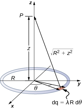
A ring has a uniform charge density \(\lambda\), with units of coulomb per unit meter of arc. Find the electric potential at a point on the axis passing through the center of the ring.

Strategy

We use the same procedure as for the charged wire. The difference here is that the charge is distributed on a circle. We divide the circle into infinitesimal elements shaped as arcs on the circle and use cylindrical coordinates shown in Figure \(\PageIndex{2}\).

Figure \(\PageIndex{2}\): We want to calculate the electric potential due to a ring of charge.

Solution

A general element of the arc between \(\theta\) and \(\theta + d\theta\) is of length \(Rd\theta\) and therefore contains a charge equal to \(\lambda Rd\theta\). The element is at a distance of \(\sqrt{z^2 + R^2}\) from \(P\), and therefore the potential is

\[\begin{align} V_p &= k\int \dfrac{dq}{r} \nonumber \\[4pt] &= k \int_0^{2\pi} \dfrac{\lambda Rd\theta}{\sqrt{z^2 + R^2}} \nonumber \\[4pt] &= \dfrac{k \lambda R}{\sqrt{z^2 + R^2}} \int_0^{2\pi} d\theta \nonumber \\[4pt] &= \dfrac{2\pi k \lambda R}{\sqrt{z^2 + R^2}} \nonumber \\[4pt] &= k \dfrac{q_{tot}}{\sqrt{z^2 + R^2}}. \nonumber \end{align} \nonumber\]

Significance

This result is expected because every element of the ring is at the same distance from point \(P\). The net potential at \(P\) is that of the total charge placed at the common distance, \(\sqrt{z^2 + R^2}\).

Example \(\PageIndex{3}\): Potential Due to a Uniform Disk of Charge

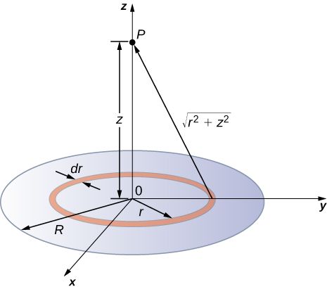
A disk of radius \(R\) has a uniform charge density \(\sigma\) with units of coulomb meter squared. Find the electric potential at any point on the axis passing through the center of the disk.

Strategy

We divide the disk into ring-shaped cells, and make use of the result for a ring worked out in the previous example, then integrate over r in addition to \(\theta\). This is shown in Figure \(\PageIndex{3}\).

Figure \(\PageIndex{3}\): We want to calculate the electric potential due to a disk of charge.

Solution

An infinitesimal width cell between cylindrical coordinates \(r\) and \(r + dr\) shown in Figure \(\PageIndex{3}\) will be a ring of charges whose electric potential \(dV_p\) at the field point has the following expression

\[dV_p = k \dfrac{dq}{\sqrt{z^2 + r^2}}\]

where

\[dq = \sigma 2\pi r dr.\]

The superposition of potential of all the infinitesimal rings that make up the disk gives the net potential at point \(P\). This is accomplished by integrating from \(r = 0\) to \(r = R\):

\[\begin{align} V_p &= \int dV_p = k2\pi \sigma \int_0^R \dfrac{r \, dr}{\sqrt{z^2 + r^2}}, \nonumber \\[4pt] &= k2\pi \sigma ( \sqrt{z^2 + R^2} - \sqrt{z^2}).\nonumber \end{align} \nonumber\]

Significance

The basic procedure for a disk is to first integrate around \(\theta\) and then over \(r\). This has been demonstrated for uniform (constant) charge density. Often, the charge density will vary with \(r\), and then the last integral will give different results.

Example \(\PageIndex{4}\): Potential Due to an Infinite Charged Wire

Find the electric potential due to an infinitely long uniformly charged wire.

Strategy

Since we have already worked out the potential of a finite wire of length \(L\) in Example \(\PageIndex{1}\), we might wonder if taking \(L \rightarrow \infty\) in our previous result will work:

\[V_p = \lim_{L \rightarrow \infty} k \lambda \ln \left(\dfrac{L + \sqrt{L^2 + 4x^2}}{-L + \sqrt{L^2 + 4x^2}}\right).\]

However, this limit does not exist because the argument of the logarithm becomes \([2/0]\) as \(L \rightarrow \infty\), so this way of finding \(V\) of an infinite wire does not work. The reason for this problem may be traced to the fact that the charges are not localized in some space but continue to infinity in the direction of the wire. Hence, our (unspoken) assumption that zero potential must be an infinite distance from the wire is no longer valid.

To avoid this difficulty in calculating limits, let us use the definition of potential by integrating over the electric field from the previous section, and the value of the electric field from this charge configuration from the previous chapter.

Solution

We use the integral

\[V_p = - \int_R^p \vec{E} \cdot d\vec{l}\]

where \(R\) is a finite distance from the line of charge, as shown in Figure \(\PageIndex{4}\).

Figure \(\PageIndex{4}\): Points of interest for calculating the potential of an infinite line of charge.

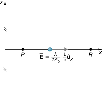
With this setup, we use \(\vec{E}_p = 2k \lambda \dfrac{1}{s} \hat{s}\) and \(d\vec{l} = d\vec{s}\) to obtain

\[\begin{align} V_p - V_R &= - \int_R^p 2k\lambda \dfrac{1}{s}ds \nonumber \\[4pt] &= -2 k \lambda \ln\dfrac{s_p}{s_R}. \nonumber \end{align} \nonumber\]

Now, if we define the reference potential \(V_R = 0\) at \(s_R = 1 \, \mathrm{m}\), this simplifies to

\[V_p = -2 k\lambda \ln s_p.\]

Note that this form of the potential is quite usable; it is 0 at 1 m and is undefined at infinity, which is why we could not use the latter as a reference.

Significance

Although calculating potential directly can be quite convenient, we just found a system for which this strategy does not work well. In such cases, going back to the definition of potential in terms of the electric field may offer a way forward.

Exercise \(\PageIndex{1}\)

What is the potential on the axis of a nonuniform ring of charge, where the charge density is \(\lambda (\theta) = \lambda \cos\theta\)?

Solution

It will be zero, as at all points on the axis, there are equal and opposite charges equidistant from the point of interest. Note that this distribution will, in fact, have a dipole moment.