3.6: Electric Potential of a Point Charge

Learning Objectives

By the end of this section, you will be able to:

• Calculate the potential due to a point charge
• Calculate the potential of a system of multiple point charges
• Calculate the potential of a continuous charge distribution

Point charges, such as electrons, are among the fundamental building blocks of matter. Furthermore, spherical charge distributions (such as charge on a metal sphere) create external electric fields exactly like a point charge. The electric potential due to a point charge is, thus, a case we need to consider.

We can use calculus to find the work needed to move a test charge \(q\) from a large distance away to a distance of \(r\) from a point charge \(q\). Noting the connection between work and potential \(W = -q\Delta V\), as in the last section, we can obtain the following result.

Electric Potential \(V\) of a Point Charge

The electric potential \(V\) of a point charge is given by

\[\underbrace{V = \dfrac{kq}{r}}_{\text{point charge}} \label{PointCharge}\]

where \(k\) is a constant equal to \(8.99 \times 10^9 \, \mathrm{N} \cdot \mathrm{m}^2/\mathrm{C}^2\).

The potential in Equation \ref{PointCharge} at infinity is chosen to be zero. Thus, \(V\) for a point charge decreases with distance, whereas \(\vec{E}\) for a point charge decreases with distance squared:

\[E = \dfrac{F}{q_t} = \dfrac{kq}{r^2}\]

Recall that the electric potential \(V\) is a scalar and has no direction, whereas the electric field \(\vec{E}\) is a vector. To find the voltage due to a combination of point charges, you add the individual voltages as numbers. To find the total electric field, you must add the individual fields as vectors, taking magnitude and direction into account. This is consistent with the fact that \(V\) is closely associated with energy, a scalar, whereas \(\vec{E}\) is closely associated with force, a vector.

Example \(\PageIndex{1}\): What Voltage Is Produced by a Small Charge on a Metal Sphere?

Charges in static electricity are typically in the nanocoulomb (nC) to microcoulomb \((\mu C)\) range. What is the voltage 5.00 cm away from the center of a 1-cm-diameter solid metal sphere that has a –3.00-nC static charge?

Strategy

As we discussed in Electric Charges and Fields, charge on a metal sphere spreads out uniformly and produces a field like that of a point charge located at its center. Thus, we can find the voltage using the equation \(V = \dfrac{kq}{r}\).

Solution

Entering known values into the expression for the potential of a point charge (Equation \ref{PointCharge}), we obtain

\[\begin{align} V &= k\dfrac{q}{r} \nonumber \\[4pt] &= (9.00 \times 10^9 \, \mathrm{N} \cdot \mathrm{m}^2/\mathrm{C}^2)\left(\dfrac{-3.00 \times 10^{-9}\mathrm{C}}{5.00 \times 10^{-2}\mathrm{m}}\right) \nonumber \\[4pt] &= - 539 \, \mathrm{V}. \nonumber \end{align} \nonumber \]

Significance

The negative value for voltage means a positive charge would be attracted from a larger distance, since the potential is lower (more negative) than at larger distances. Conversely, a negative charge would be repelled, as expected.

Example \(\PageIndex{2}\): What Is the Excess Charge on a Van de Graaff Generator?

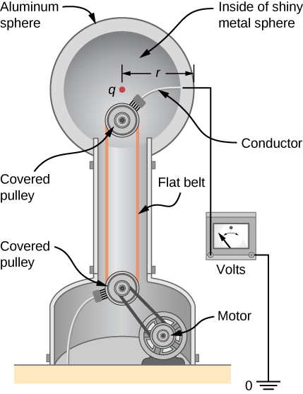
A demonstration Van de Graaff generator has a 25.0-cm-diameter metal sphere that produces a voltage of 100 kV near its surface (Figure). What excess charge resides on the sphere? (Assume that each numerical value here is shown with three significant figures.)

Figure \(\PageIndex{1}\): The voltage of this demonstration Van de Graaff generator is measured between the charged sphere and ground. Earth’s potential is taken to be zero as a reference. The potential of the charged conducting sphere is the same as that of an equal point charge at its center.

Strategy

The potential on the surface is the same as that of a point charge at the center of the sphere, 12.5 cm away. (The radius of the sphere is 12.5 cm.) We can thus determine the excess charge using Equation \ref{PointCharge}

\[V = \dfrac{kq}{r}.\]

Solution

Solving for \(q\) and entering known values gives

\[\begin{align} q &= \dfrac{rV}{k} \nonumber \\[4pt] &= \dfrac{(0.125 \, \mathrm{m})(100 \times 10^3 \, \mathrm{V})}{8.99 \times 10^9\,\mathrm{N} \cdot \mathrm{m}^2/\mathrm{C}^2} \nonumber \\[4pt] &= 1.39 \times 10^{-6}\,\mathrm{C} \nonumber \\[4pt] &= 1.39 \, \mu\mathrm{C}. \nonumber \end{align} \nonumber

Significance

This is a relatively small charge, but it produces a rather large voltage. We have another indication here that it is difficult to store isolated charges.

Exercise \(\PageIndex{1}\)

What is the potential inside the metal sphere in Example \(\PageIndex{1}\)?

Answer

\[\begin{align} V &= k\dfrac{q}{r} \nonumber \\[4pt] &= (8.99 \times 10^9\,\mathrm{N} \cdot \mathrm{m}^2/\mathrm{C}^2) \left(\dfrac{-3.00 \times 10^{-9}\,\mathrm{C}}{5.00 \times 10^{-3}\,\mathrm{m}}\right) \nonumber \\[4pt] &= - 5390 \, \mathrm{V}\nonumber \end{align} \nonumber \]

Recall that the electric field inside a conductor is zero. Hence, any path from a point on the surface to any point in the interior will have an integrand of zero when calculating the change in potential, and thus the potential in the interior of the sphere is identical to that on the surface.

The voltages in both of these examples could be measured with a meter that compares the measured potential with ground potential. Ground potential is often taken to be zero (instead of taking the potential at infinity to be zero). It is the potential difference between two points that is of importance, and very often there is a tacit assumption that some reference point, such as Earth or a very distant point, is at zero potential. As noted earlier, this is analogous to taking sea level as \(h = 0\) when considering gravitational potential energy \(U_g = mgh\).

Systems of Multiple Point Charges

Just as the electric field obeys a superposition principle, so does the electric potential. Consider a system consisting of \(N\) charges \(q_1,q_2,. . ., q_N\). What is the net electric potential \(V\) at a space point \(P\) from these charges? Each of these charges is a source charge that produces its own electric potential at point \(P\), independent of whatever other changes may be doing. Let \(V_1, V_2, . . ., V_N\) be the electric potentials at \(P\) produced by the charges \(q_1,q_2,. . ., q_N\), respectively. Then, the net electric potential \(V_p\) at that point is equal to the sum of these individual electric potentials. You can easily show this by calculating the potential energy of a test charge when you bring the test charge from the reference point at infinity to point \(P\):

\[V_p = V_1 + V_2 + . . . + V_N = \sum_1^N V_i.\]

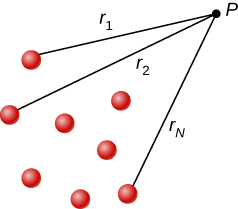
Note that electric potential follows the same principle of superposition as electric field and electric potential energy. To show this more explicitly, note that a test charge \(q_i\) at the point \(P\) in space has distances of \(r_1,r_2, . . . ,r_N\) from the \(N\), charges fixed in space above, as shown in Figure \(\PageIndex{2}\). Using our formula for the potential of a point charge for each of these (assumed to be point) charges, we find that

\[V_p = \sum_1^N k\dfrac{q_i}{r_i} = k\sum_1^N \dfrac{q_i}{r_i}. \label{eq20}\]

Therefore, the electric potential energy of the test charge is

\[U_p = q_tV_p = q_tk\sum_1^N \dfrac{q_i}{r_i},\] which is the same as the work to bring the test charge into the system, as found in the first section of the chapter.

Figure \(\PageIndex{2}\): Notation for direct distances from charges to a space point \(P\).

 An electric dipole is a system of two equal but opposite charges a fixed distance apart. This system is used to model many real-world systems, including atomic and molecular interactions. One of these systems is the water molecule, under certain circumstances. These circumstances are met inside a microwave oven, where electric fields with alternating directions make the water molecules change orientation. This vibration is the same as heat  at the molecular level.

Example \(\PageIndex{3}\): Electric Potential of a Dipole

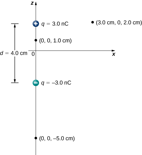
Consider the dipole in Figure \(\PageIndex{3}\) with the charge magnitude of \(q = 3.0 \, \mu \mathrm{C}\) and separation distance \(d = 4.0 \, \mathrm{cm}.\) What is the potential at the following locations in space? (a) (0, 0, 1.0 cm); (b) (0, 0, –5.0 cm); (c) (3.0 cm, 0, 2.0 cm).

Figure \(\PageIndex{3}\): A general diagram of an electric dipole, and the notation for the distances from the individual charges to a point \(P\) in space.

Strategy

Apply \(V_p = k \sum_1^N \dfrac{q_i}{r_i}\) to each of these three points.

Solution

a. \(V_p = k \sum_1^N \dfrac{q_i}{r_i} = (9.0 \times 10^9 \,\textrm{N} \cdot \textrm{m}^2/\textrm{C}^2) \left(\dfrac{3.0\space \textrm{nC}}{0.010 \, \textrm{m}} - \dfrac{3.0\space \textrm{nC}}{0.030 \, \textrm{m}}\right) = 1.8 \times 10^3 \, \textrm{V}\)

b. \(V_p = k \sum_1^N \dfrac{q_i}{r_i} = (9.0 \times 10^9 \, \textrm{N} \cdot \textrm{m}^2/\textrm{C}^2) \left(\dfrac{3.0\space \textrm{nC}}{0.070 \, \textrm{m}} - \dfrac{3.0\space \textrm{nC}}{0.030 \, \textrm{m}}\right) = -5.1 \times 10^2 \, \textrm{V}\)

c. \(V_p = k \sum_1^N \dfrac{q_i}{r_i} = (9.0 \times 10^9 \, \textrm{N} \cdot \textrm{m}^2/\textrm{C}^2) \left(\dfrac{3.0\space \textrm{nC}}{0.030 \, \textrm{m}} - \dfrac{3.0\space \textrm{nC}}{0.050 \, \textrm{m}}\right) = 3.6 \times 10^2 \, \textrm{V}\)

Significance

Note that evaluating potential is significantly simpler than electric field, due to potential being a scalar instead of a vector.

Exercise \(\PageIndex{1}\)

What is the potential on the \(x\)-axis? The \(z\)-axis?

Answer

The \(x\)-axis the potential is zero, due to the equal and opposite charges the same distance from it. On the \(z\)-axis, we may superimpose the two potentials; we will find that for \(z > > d\), again the potential goes to zero due to cancellation.