
6.2: Source Voltage


- Last updated
- Nov 10, 2024
- Save as PDF
( \newcommand{\kernel}{\mathrm{null}\,}\)
By the end of the section, you will be able to:
- Describe the source voltage and the internal resistance of a battery.
- Explain the basic operation of a battery.
If you forget to turn off your car lights, they slowly dim as the battery runs down. Why don’t they suddenly blink off when the battery’s energy is gone? Their gradual dimming implies that the battery output voltage decreases as the battery is depleted. The reason for the decrease in output voltage for depleted batteries is that all voltage sources have two fundamental parts—a source of electrical energy and an internal resistance. In this section, we examine the energy source and the internal resistance.
Introduction to Source Voltage
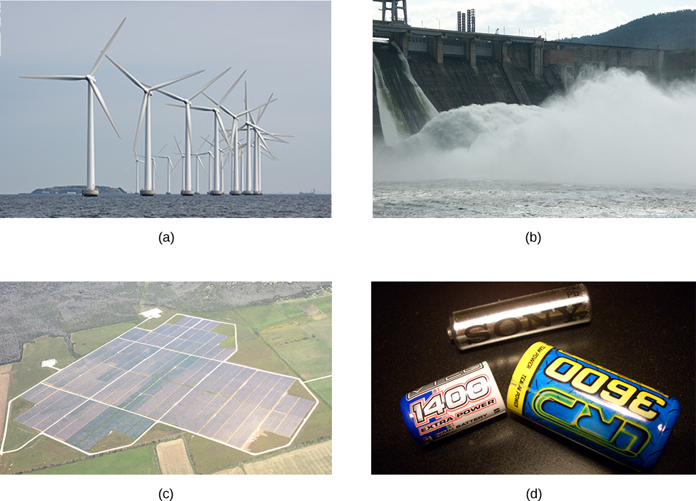
Voltage has many sources, a few of which are shown in Figure 6.2.2. All such devices create a potential difference and can supply current if connected to a circuit. A special type of potential difference is known as source voltage. (Note: Source voltage is called electromotive force (emf) in some text, but this usage is deprecated because emf is not a force and does not have dimensions of newtons in the SI system.)
Consider a simple circuit of a 12-V lamp attached to a 12-V battery, as shown in Figure 6.2.2. The battery can be modeled as a two-terminal device that keeps one terminal at a higher electric potential than the second terminal. The higher electric potential is sometimes called the positive terminal and is labeled with a plus sign. The lower-potential terminal is sometimes called the negative terminal and labeled with a minus sign.
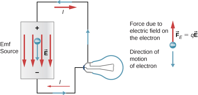
When the battery is not connected to the lamp, there is no net flow of charge within the battery. Once the battery is connected to the lamp, charges flow from one terminal of the battery, through the lamp (causing the lamp to light), and back to the other terminal of the battery. If we consider positive (conventional) current flow, positive charges leave the positive terminal, travel through the lamp, and enter the negative terminal.
Positive current flow is useful for most of the circuit analysis in this chapter, but in metallic wires and resistors, electrons contribute the most to current, flowing in the opposite direction of positive current flow. Therefore, it is more realistic to consider the movement of electrons for the analysis of the circuit in Figure 6.2.2. The electrons leave the negative terminal, travel through the lamp, and return to the positive terminal. For the battery to maintain the potential difference between the two terminals, negative charges (electrons) must be moved from the positive terminal to the negative terminal. The battery acts as a charge pump, moving negative charges from the positive terminal to the negative terminal to maintain the potential difference. This increases the potential energy of the charges and, therefore, the electric potential of the charges.
The force on the negative charge from the electric field is in the opposite direction of the electric field, as shown in Figure 6.2.2. For the negative charges to be moved to the negative terminal, work must be done on the negative charges. This requires energy, which comes from chemical reactions in the battery. The potential is kept high on the positive terminal and low on the negative terminal to maintain the potential difference between the two terminals. The source voltage is equal to the work done on the charge per unit charge (ε=dWdq) when there is no current flowing. Since the unit for work is the joule and the unit for charge is the coulomb, the unit for source voltage is the volt (1V=1J/C).
The terminal voltage Vterminal of a battery is the voltage measured across the terminals of the battery when there is no load connected to the terminal. An ideal battery maintains a constant terminal voltage, independent of the current between the two terminals. An ideal battery has no internal resistance, and the terminal voltage is equal to the source voltage of the battery. In the next section, we will show that a real battery does have internal resistance and the terminal voltage is always less than the source voltage of the battery.
The Origin of Battery Potential
The first battery was invented in 1799 by Alessandro Volta and was also known as the voltaic pile. Modern batteries have improved considerably since those early times, but often still retain the concept of a series of cells, each of which creates a potential difference. The combination of chemicals and the makeup of the terminals in a battery determine its source voltage. The lead acid battery used in cars and other vehicles is one of the most common combinations of chemicals. Figure 6.2.3 shows a single cell (one of six) of this battery. The cathode (positive) terminal of the cell is connected to a lead oxide plate, whereas the anode (negative) terminal is connected to a lead plate. Both plates are immersed in sulfuric acid, the electrolyte for the system.

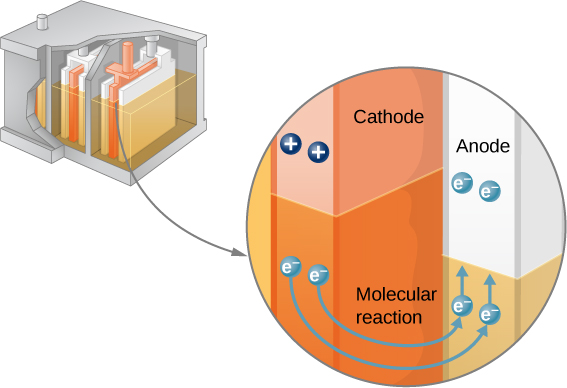
Knowing a little about how the chemicals in a lead-acid battery interact helps in understanding the potential created by the battery. Figure 6.2.4 shows the result of a single chemical reaction. Two electrons are placed on the anode, making it negative, provided that the cathode supplies two electrons. This leaves the cathode positively charged, because it has lost two electrons. In short, a separation of charge has been driven by a chemical reaction.
Note that the reaction does not take place unless there is a complete circuit to allow two electrons to be supplied to the cathode. Under many circumstances, these electrons come from the anode, flow through a resistance, and return to the cathode. Note also that since the chemical reactions involve substances with resistance, it is not possible to create the source voltage without an internal resistance.
Internal Resistance and Terminal Voltage
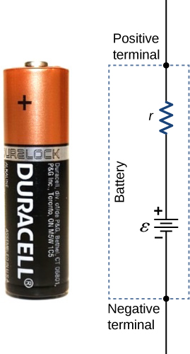
The amount of resistance to the flow of current within the voltage source is called the internal resistance. The internal resistance r of a battery can behave in complex ways. It generally increases as a battery is depleted, due to the oxidation of the plates or the reduction of the acidity of the electrolyte. However, internal resistance may also depend on the magnitude and direction of the current through a voltage source, its temperature, and even its history. The internal resistance of rechargeable nickel-cadmium cells, for example, depends on how many times and how deeply they have been depleted. A simple model for a battery consists of an idealized source voltage ε and an internal resistance r (Figure 6.2.5).
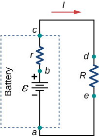
Suppose an external resistor, known as the load resistance R, is connected to a voltage source such as a battery, as in Figure 6.2.6. The figure shows a model of a battery with a source voltage ε, an internal resistance r, and a load resistor R connected across its terminals. Using conventional current flow, positive charges leave the positive terminal of the battery, travel through the resistor, and return to the negative terminal of the battery. The terminal voltage of the battery depends on the source voltage, the internal resistance, and the current, and is equal to
Vterminal=ε−Ir
For a given source voltage and internal resistance, the terminal voltage decreases as the current increases due to the potential drop Ir of the internal resistance.
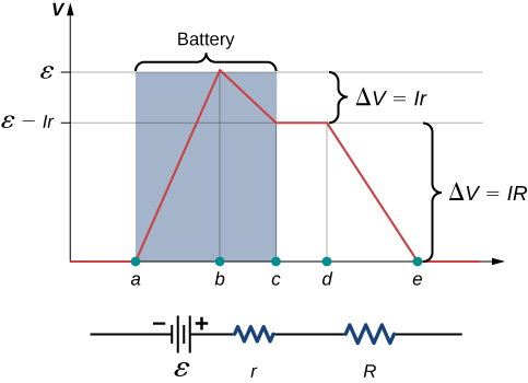
A graph of the potential difference across each element the circuit is shown in Figure 6.2.7. A current I runs through the circuit, and the potential drop across the internal resistor is equal to Ir. The terminal voltage is equal to ε−Ir, which is equal to the potential drop across the load resistor IR=ε−Ir. As with potential energy, it is the change in voltage that is important. When the term “voltage” is used, we assume that it is actually the change in the potential, or ΔV. However, Δ is often omitted for convenience.
The current through the load resistor is I=εr+R. We see from this expression that the smaller the internal resistance r, the greater the current the voltage source supplies to its load R. As batteries are depleted, r increases. If r becomes a significant fraction of the load resistance, then the current is significantly reduced, as the following example illustrates.
A given battery has a 12.00-V source voltage and an internal resistance of 0.100Ω. (a) Calculate its terminal voltage when connected to a10.00Ω load. (b) What is the terminal voltage when connected to a 0.500Ω load? (c) What power does the 0.500Ω load dissipate? (d) If the internal resistance grows to 0.500Ω, find the current, terminal voltage, and power dissipated by a 0.500Ω load.
Strategy
The analysis above gave an expression for current when internal resistance is taken into account. Once the current is found, the terminal voltage can be calculated by using the equation Vterminal=ε−Ir. Once current is found, we can also find the power dissipated by the resistor.
Solution
- Entering the given values for the source voltage, load resistance, and internal resistance into the expression above yields I=εR+r=12.00V10.10Ω=1.188A. Enter the known values into the equationVterminal=ε−Ir to get the terminal voltage: Vterminal=ε−Ir=12.00V−(1.188A)(0.100Ω)=11.90V. The terminal voltage here is only slightly lower than the source voltage, implying that the current drawn by this light load is not significant.
- Similarly, with Rload=0.500Ω, the current is I=εR+r=12.00V0.600Ω=20.00A. The terminal voltage is now Vterminal=ε−Ir=12.00V−(20.00A)(0.100Ω)=10.00V. The terminal voltage exhibits a more significant reduction compared with source voltage, implying 0.500Ω is a heavy load for this battery. A “heavy load” signifies a larger draw of current from the source but not a larger resistance.
- The power dissipated by the 0.500Ω load can be found using the formula P=I2R. Entering the known values gives P=I2R=(20.0A)2(0.500Ω)=2.00×10²W. Note that this power can also be obtained using the expression V2R or IV, where V is the terminal voltage (10.0 V in this case).
- Here, the internal resistance has increased, perhaps due to the depletion of the battery, to the point where it is as great as the load resistance. As before, we first find the current by entering the known values into the expression, yielding I=εR+r=12.00V1.00Ω=12.00A. Now the terminal voltage is Vterminal=ε−Ir=12.00V−(12.00A)(0.500Ω)=6.00V, and the power dissipated by the load is P=I2R=(12.00A)2(0.500Ω)=72.00W. We see that the increased internal resistance has significantly decreased the terminal voltage, current, and power delivered to a load.
Significance
The internal resistance of a battery can increase for many reasons. For example, the internal resistance of a rechargeable battery increases as the number of times the battery is recharged increases. The increased internal resistance may have two effects on the battery. First, the terminal voltage will decrease. Second, the battery may overheat due to the increased power dissipated by the internal resistance.
If you place a wire directly across the two terminal of a battery, effectively shorting out the terminals, the battery will begin to get hot. Why do you suppose this happens?
- Solution
-
If a wire is connected across the terminals, the load resistance is close to zero, or at least considerably less than the internal resistance of the battery. Since the internal resistance is small, the current through the circuit will be large, I=εR+r=ε0+r=εr. The large current causes a high power to be dissipated by the internal resistance (P=I2r). The power is dissipated as heat.
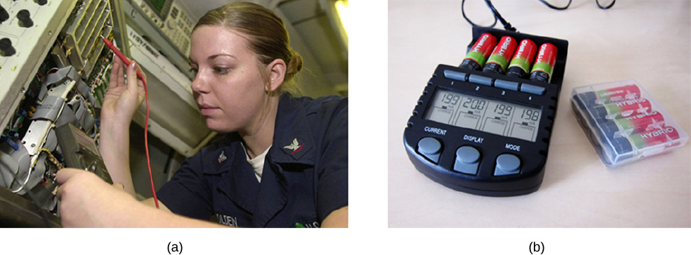
Battery Testers
Battery testers, such as those in Figure 6.2.8, use small load resistors to intentionally draw current to determine whether the terminal potential drops below an acceptable level. Although it is difficult to measure the internal resistance of a battery, battery testers can provide a measurement of the internal resistance of the battery. If internal resistance is high, the battery is weak, as evidenced by its low terminal voltage.
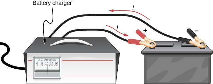
Some batteries can be recharged by passing a current through them in the direction opposite to the current they supply to an appliance. This is done routinely in cars and in batteries for small electrical appliances and electronic devices (Figure 6.2.9). The voltage output of the battery charger must be greater than the source voltage of the battery to reverse the current through it. This causes the terminal voltage of the battery to be greater than the source voltage, since V=ε−Ir and I is now negative.
It is important to understand the consequences of the internal resistance of devices which provide source voltage, such as batteries and solar cells, but often, the analysis of circuits is done with the terminal voltage of the battery, as we have done in the previous sections. The terminal voltage is referred to as simply as V, dropping the subscript “terminal.” This is because the internal resistance of the battery is difficult to measure directly and can change over time.
Contributors and Attributions
Samuel J. Ling (Truman State University), Jeff Sanny (Loyola Marymount University), and Bill Moebs with many contributing authors. This work is licensed by OpenStax University Physics under a Creative Commons Attribution License (by 4.0).