Physics LibreTexts

16.6: Direct Calculation of Electrical Quantities from Charge Distributions (Exercises)

  • Page ID
    100312
  • \( \newcommand{\vecs}[1]{\overset { \scriptstyle \rightharpoonup} {\mathbf{#1}} } \)

    \( \newcommand{\vecd}[1]{\overset{-\!-\!\rightharpoonup}{\vphantom{a}\smash {#1}}} \)

    \( \newcommand{\id}{\mathrm{id}}\) \( \newcommand{\Span}{\mathrm{span}}\)

    ( \newcommand{\kernel}{\mathrm{null}\,}\) \( \newcommand{\range}{\mathrm{range}\,}\)

    \( \newcommand{\RealPart}{\mathrm{Re}}\) \( \newcommand{\ImaginaryPart}{\mathrm{Im}}\)

    \( \newcommand{\Argument}{\mathrm{Arg}}\) \( \newcommand{\norm}[1]{\| #1 \|}\)

    \( \newcommand{\inner}[2]{\langle #1, #2 \rangle}\)

    \( \newcommand{\Span}{\mathrm{span}}\)

    \( \newcommand{\id}{\mathrm{id}}\)

    \( \newcommand{\Span}{\mathrm{span}}\)

    \( \newcommand{\kernel}{\mathrm{null}\,}\)

    \( \newcommand{\range}{\mathrm{range}\,}\)

    \( \newcommand{\RealPart}{\mathrm{Re}}\)

    \( \newcommand{\ImaginaryPart}{\mathrm{Im}}\)

    \( \newcommand{\Argument}{\mathrm{Arg}}\)

    \( \newcommand{\norm}[1]{\| #1 \|}\)

    \( \newcommand{\inner}[2]{\langle #1, #2 \rangle}\)

    \( \newcommand{\Span}{\mathrm{span}}\) \( \newcommand{\AA}{\unicode[.8,0]{x212B}}\)

    \( \newcommand{\vectorA}[1]{\vec{#1}}      % arrow\)

    \( \newcommand{\vectorAt}[1]{\vec{\text{#1}}}      % arrow\)

    \( \newcommand{\vectorB}[1]{\overset { \scriptstyle \rightharpoonup} {\mathbf{#1}} } \)

    \( \newcommand{\vectorC}[1]{\textbf{#1}} \)

    \( \newcommand{\vectorD}[1]{\overrightarrow{#1}} \)

    \( \newcommand{\vectorDt}[1]{\overrightarrow{\text{#1}}} \)

    \( \newcommand{\vectE}[1]{\overset{-\!-\!\rightharpoonup}{\vphantom{a}\smash{\mathbf {#1}}}} \)

    \( \newcommand{\vecs}[1]{\overset { \scriptstyle \rightharpoonup} {\mathbf{#1}} } \)

    \( \newcommand{\vecd}[1]{\overset{-\!-\!\rightharpoonup}{\vphantom{a}\smash {#1}}} \)

    \(\newcommand{\avec}{\mathbf a}\) \(\newcommand{\bvec}{\mathbf b}\) \(\newcommand{\cvec}{\mathbf c}\) \(\newcommand{\dvec}{\mathbf d}\) \(\newcommand{\dtil}{\widetilde{\mathbf d}}\) \(\newcommand{\evec}{\mathbf e}\) \(\newcommand{\fvec}{\mathbf f}\) \(\newcommand{\nvec}{\mathbf n}\) \(\newcommand{\pvec}{\mathbf p}\) \(\newcommand{\qvec}{\mathbf q}\) \(\newcommand{\svec}{\mathbf s}\) \(\newcommand{\tvec}{\mathbf t}\) \(\newcommand{\uvec}{\mathbf u}\) \(\newcommand{\vvec}{\mathbf v}\) \(\newcommand{\wvec}{\mathbf w}\) \(\newcommand{\xvec}{\mathbf x}\) \(\newcommand{\yvec}{\mathbf y}\) \(\newcommand{\zvec}{\mathbf z}\) \(\newcommand{\rvec}{\mathbf r}\) \(\newcommand{\mvec}{\mathbf m}\) \(\newcommand{\zerovec}{\mathbf 0}\) \(\newcommand{\onevec}{\mathbf 1}\) \(\newcommand{\real}{\mathbb R}\) \(\newcommand{\twovec}[2]{\left[\begin{array}{r}#1 \\ #2 \end{array}\right]}\) \(\newcommand{\ctwovec}[2]{\left[\begin{array}{c}#1 \\ #2 \end{array}\right]}\) \(\newcommand{\threevec}[3]{\left[\begin{array}{r}#1 \\ #2 \\ #3 \end{array}\right]}\) \(\newcommand{\cthreevec}[3]{\left[\begin{array}{c}#1 \\ #2 \\ #3 \end{array}\right]}\) \(\newcommand{\fourvec}[4]{\left[\begin{array}{r}#1 \\ #2 \\ #3 \\ #4 \end{array}\right]}\) \(\newcommand{\cfourvec}[4]{\left[\begin{array}{c}#1 \\ #2 \\ #3 \\ #4 \end{array}\right]}\) \(\newcommand{\fivevec}[5]{\left[\begin{array}{r}#1 \\ #2 \\ #3 \\ #4 \\ #5 \\ \end{array}\right]}\) \(\newcommand{\cfivevec}[5]{\left[\begin{array}{c}#1 \\ #2 \\ #3 \\ #4 \\ #5 \\ \end{array}\right]}\) \(\newcommand{\mattwo}[4]{\left[\begin{array}{rr}#1 \amp #2 \\ #3 \amp #4 \\ \end{array}\right]}\) \(\newcommand{\laspan}[1]{\text{Span}\{#1\}}\) \(\newcommand{\bcal}{\cal B}\) \(\newcommand{\ccal}{\cal C}\) \(\newcommand{\scal}{\cal S}\) \(\newcommand{\wcal}{\cal W}\) \(\newcommand{\ecal}{\cal E}\) \(\newcommand{\coords}[2]{\left\{#1\right\}_{#2}}\) \(\newcommand{\gray}[1]{\color{gray}{#1}}\) \(\newcommand{\lgray}[1]{\color{lightgray}{#1}}\) \(\newcommand{\rank}{\operatorname{rank}}\) \(\newcommand{\row}{\text{Row}}\) \(\newcommand{\col}{\text{Col}}\) \(\renewcommand{\row}{\text{Row}}\) \(\newcommand{\nul}{\text{Nul}}\) \(\newcommand{\var}{\text{Var}}\) \(\newcommand{\corr}{\text{corr}}\) \(\newcommand{\len}[1]{\left|#1\right|}\) \(\newcommand{\bbar}{\overline{\bvec}}\) \(\newcommand{\bhat}{\widehat{\bvec}}\) \(\newcommand{\bperp}{\bvec^\perp}\) \(\newcommand{\xhat}{\widehat{\xvec}}\) \(\newcommand{\vhat}{\widehat{\vvec}}\) \(\newcommand{\uhat}{\widehat{\uvec}}\) \(\newcommand{\what}{\widehat{\wvec}}\) \(\newcommand{\Sighat}{\widehat{\Sigma}}\) \(\newcommand{\lt}{<}\) \(\newcommand{\gt}{>}\) \(\newcommand{\amp}{&}\) \(\definecolor{fillinmathshade}{gray}{0.9}\)

    Conceptual Questions

    Electric Dipoles

    36. What are the stable orientation(s) for a dipole in an external electric field? What happens if the dipole is slightly perturbed from these orientations?

    Calculating Electric Potential of Charge Distributions

    13. Compare the electric dipole moments of charges \(\displaystyle ±Q\) separated by a distance d and charges \(\displaystyle ±Q/2\) separated by a distance d/2.

    15. In what region of space is the potential due to a uniformly charged sphere the same as that of a point charge? In what region does it differ from that of a point charge?

    16. Can the potential of a nonuniformly charged sphere be the same as that of a point charge? Explain.

    Problems

    Electric Dipoles

    105. Consider the equal and opposite charges shown below. (a) Show that at all points on the x-axis for which \(\displaystyle |x|≫a,E≈Qa/2πε_0x^3\). (b) Show that at all points on the y-axis for which \(\displaystyle |y|≫a,E≈Qa/πε_0y^3\).

    Two charges are shown on the y axis of an x y coordinate system. Charge +Q is a distance a above the origin, and charge −Q is a distance a below the origin.

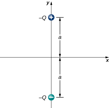
    106. (a) What is the dipole moment of the configuration shown above? If Q=4.0μC,

    (b) what is the torque on this dipole with an electric field of \(\displaystyle 4.0×10^5N/C\hat{i}\)?

    (c) What is the torque on this dipole with an electric field of \(\displaystyle −4.0×10^5N/C\hat{i}\)?

    (d) What is the torque on this dipole with an electric field of \(\displaystyle ±4.0×10^5N/C\hat{j}\)?

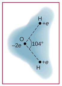
    107. A water molecule consists of two hydrogen atoms bonded with one oxygen atom. The bond angle between the two hydrogen atoms is 104° (see below). Calculate the net dipole moment of a hypothetical water molecule where the charge at the oxygen molecule is −2e and at each hydrogen atom is +e. The net dipole moment of the molecule is the vector sum of the individual dipole moment between the two O-Hs. The separation O-H is 0.9578 angstroms.

    A schematic representation of the outer electron cloud of a neutral water molecule is shown. Three atoms are at the vertices of a triangle. The hydrogen atom has positive q charge and the oxygen atom has minus two q charge, and the angle between the line joining each hydrogen atom with the oxygen atom is one hundred and four degrees. The cloud density is shown as being greater at the oxygen atom.

    Calculating Electric Fields of Charge Distributions

    83. The charge per unit length on the thin rod shown below is \(\displaystyle λ\). What is the electric field at the point P? (Hint: Solve this problem by first considering the electric field \(\displaystyle d\vec{E}\) at P due to a small segment dx of the rod, which contains charge \(\displaystyle dq=λdx\). Then find the net field by integrating \(\displaystyle d\vec{E}\) over the length of the rod.)

    A horizontal rod of length L is shown. The rod has total charge q. Point P is a distance a to the right of the right end of the rod.

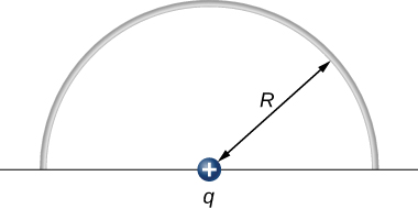
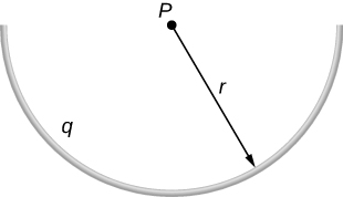
    84. The charge per unit length on the thin semicircular wire shown below is λ. What is the electric field at the point P?

    A semicircular arc of radius r is shown. The arc has total charge q. Point P is at the center of the circle of which the arc is a part.

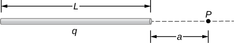
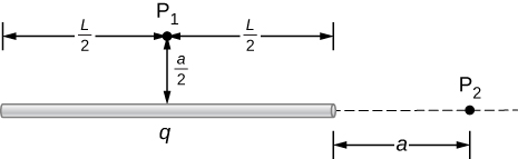
    87. A total charge q is distributed uniformly along a thin, straight rod of length L (see below). What is the electric field at \(\displaystyle P_1\)? At \(\displaystyle P_2\)?

    A horizontal rod of length L is shown. The rod has total charge q. Point P 1 is a distance a over 2 above the midpoint of the rod, so that the horizontal distance from P 1 to each end of the rod is L over 2. Point P 2 is a distance a to the right of the right end of the rod.

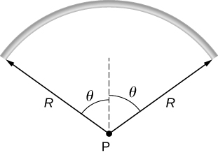
    90. A rod bent into the arc of a circle subtends an angle \(\displaystyle 2θ\) at the center P of the circle (see below). If the rod is charged uniformly with a total charge Q, what is the electric field at P?.

    An arc that is part of a circle of radius R and with center P is shown. The arc extends from an angle theta to the left of vertical to an angle theta to the right of vertical.

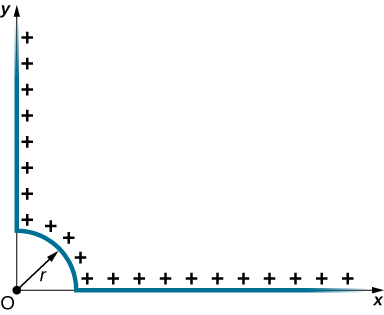
    97. Positive charge is distributed with a uniform density \(\displaystyle λ\) along the positive x-axis from \(\displaystyle r\) to \(\displaystyle ∞\), along the positive y-axis from \(\displaystyle r\) to \(\displaystyle ∞\), and along a 90° arc of a circle of radius r, as shown below. What is the electric field at O?

    A uniform distribution of positive charges is shown on an x y coordinate system. The charges are distributed along a 90 degree arc of a circle of radius r in the first quadrant, centered on the origin. The distribution continues along the positive x and y axes from r to infinity.

    121. Charge is distributed uniformly along the entire y-axis with a density \(\displaystyle y_λ\) and along the positive x-axis from \(\displaystyle x=a\) to \(\displaystyle x=b\) with a density \(\displaystyle λ_x\). What is the force between the two distributions?

    122. The circular arc shown below carries a charge per unit length \(\displaystyle λ=λ_0cosθ\), where \(\displaystyle θ\) is measured from the x-axis. What is the electric field at the origin?

    123. Calculate the electric field due to a uniformly charged rod of length L, aligned with the x-axis with one end at the origin; at a point P on the z-axis.

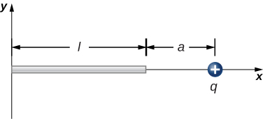
    124. The charge per unit length on the thin rod shown below is \(\displaystyle λ\). What is the electric force on the point charge q? Solve this problem by first considering the electric force \(\displaystyle d\vec{F}\) on q due to a small segment \(\displaystyle dx\) of the rod, which contains charge \(\displaystyle λdx.\) Then, find the net force by integrating \(\displaystyle d\vec{F}\) over the length of the rod.

    A rod of length l is shown. The rod lies on the horizontal axis, with its left end at the origin. A positive charge q is on the x axis, a distance a to the right of the right end of the rod.

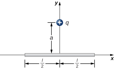
    125. The charge per unit length on the thin rod shown here is \(\displaystyle λ\). What is the electric force on the point charge q? (See the preceding problem.)

    A rod of length l is shown. The rod lies on the horizontal axis, with its center at the origin, so the ends are a distance of l over 2 to the left and right of the origin. A positive charge q is on the y axis, a distance a to above the origin.

    126. The charge per unit length on the thin semicircular wire shown below is \(\displaystyle λ\). What is the electric force on the point charge q? (See the preceding problems.)

    A semicircular arc that the upper half of a circle of radius R is shown. A positive charge q is at the center of the circle.


    16.6: Direct Calculation of Electrical Quantities from Charge Distributions (Exercises) is shared under a not declared license and was authored, remixed, and/or curated by LibreTexts.