
16.7: Direct Calculation of Electrical Quantities from Charge Distributions (Answers)
( \newcommand{\kernel}{\mathrm{null}\,}\)
Note: Answers are provided for only the odd-numbered questions.
Conceptual Questions
Calculating Electric Potential of Charge Distributions
13. The second has 1/4 the dipole moment of the first.
15. The region outside of the sphere will have a potential indistinguishable from a point charge; the interior of the sphere will have a different potential.
Problems
Electric Dipoles
105. Ex=0,Ey=14πε0[2q(x2+a2)a√(x2+a2)⇒x≫a⇒12πε0qax3
Ey=q4πε0[2ya+2ya(y−a)2(y+a)2]⇒y≫a⇒1πε0qay3
107. The net dipole moment of the molecule is the vector sum of the individual dipole moments between the two O-H. The separation O-H is 0.9578 angstroms:
→p=1.889×10⁻²⁹Cmˆi
Calculating Electric Fields of Charge Distributions
83. dE=14πε0λdx(x+a)2,E=λ4πε0[1l+a−1a]
87. At P1:→E(y)=14πε0λLy√y2+L24ˆj⇒14πε0qa2√(a2)2+L24ˆj=1πε0qa√a2+L2ˆj
At P2: Put the origin at the end of L.
dE=14πε0λdx(x+a)2,→E=−q4πε0l[1l+a−1a]ˆi
97. circular arc dEx(−ˆi)=14πε0λdsr2cosθ(−ˆi,
→Ex=λ4πε0r(−ˆi),
dEy(−ˆiˆ)=14πε0λdsr2sinθ(−ˆj),
→Ey=λ4πε0r(−ˆj);
y-axis: →Ex=λ4πε0r(−ˆi);
x-axis: →Ey=λ4πε0r(−ˆj),
→E=λ2πε0r(−ˆi)+λ2πε0r(−ˆj)
Additional Problems
121. Electric field of wire at x: →E(x)=14πε02λyxˆi,
dF=λyλx2πε0(lnb−lna)
123.
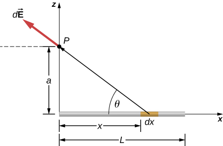
dEx=14πε0λdx(x2+a2)x√x2+a2,
→Ex=λ4πε0[1√L2+a2−1a]ˆi,
dEz=14πε0λdx(x2+a2)a√x2+a2,
→Ez=λ4πε0aL√L2+a2ˆk,
Substituting z for a, we have:
→E(z)=λ4πε0[1√L2+z2−1z]ˆi+λ4πε0zL√L2+z2ˆk
125. There is a net force only in the y-direction. Let θ be the angle the vector from dx to q makes with the x-axis. The components along the x-axis cancel due to symmetry, leaving the y-component of the force.
dFy=14πε0aqλdx(x2+a2)3/2,
Fy=12πε0qλa[l/2((l/2)2+a2)1/2]