7.2: The Friedmann-Lemaitre-Robertson-Walker Metric

Solving the Einstein Field Equations given the conditions that the universe is homogeneous and isotropic yields what we call the Friedmann-Lemaitre-Robertson-Walker (FLRW) Metric, named after four scientists who each made individual contributions. It can be written as

\[d\tau^2=dt^2-a^2(t)\left (dr^2+S^2(r)\left (d\theta^2+\sin^2\theta d\phi^2\right)\right)\label{eq:FLRW},\]

where

\[S(r)=\begin{cases} R\sin\left(\frac{r}{R}\right) & \text{spatial geometry: sphere}\\ r & \text{spatial geometry: flat}\\ R\sinh\left(\frac{r}{R}\right)&\text{spatial geometry: saddle-like}\end{cases}\]

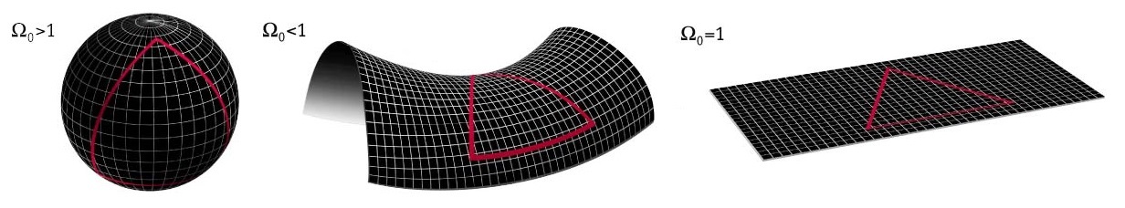
and where \(R\) represents the radius of curvature of the universe, and \(a(t)\) is called the scale factor. Note that the function \(S(r)\) depends on the overall curvature of the universe, as depicted in Figure \(\PageIndex{1}\). The overall curvature, as we will see later, depends on the density of all of the stuff in the universe. I would also like to point out that sphere, flat, and saddle-like refer to the rules of geometry and do not mean that all of the stuff in the universe is arranged in such a way as to look like it all falls on the surface of a sphere, a plane, or a saddle.

Figure \(\PageIndex{1}\): Three possible geometries of the universe. In a spherical universe (top), the three angles of a triangle add up to more than 180 degrees. In a saddle-like universe (middle), the three angles of a triangle add up to less than 180 degrees. In a flat universe, the three angles of a triangle add up to 180 degrees. (Image credit: Wikipedia)

In practice, \(S(r)\) is not that important to us. It only affects how we calculate the lengths of arcs on the sky. Astronomy, however, is done by looking at light that travels radially toward us (we are always free to choose ourselves as the origin of the coordinate system).

Exercise \(\PageIndex{1}\)

Suppose we had a dial that could control the value of \(R\). In principle, we should be able to dial up or dial down the value of \(R\) and eventually produce a spatially flat geometry. What \(R\) value achieves that?

Answer

Since \(R\) represents the spatial curvature of the universe, it would make sense that \(R\to \infty\) should yield a flat universe. While you may think that \(\lim_\limits{R\to \infty}R\sin\left(\frac{r}{R}\right)=0\), it actually turns out that \(\lim_\limits{R\to \infty}R\sin\left(\frac{r}{R}\right)=r\). The same is true for \(R\sinh\left(\frac{r}{R}\right )\). In both cases, the limit \(R\to \infty\) reduces to the expression for \(S(r)\) for a flat geometry.

Exercise \(\PageIndex{2}\)

If you were to draw a triangle on a piece of paper and measure the three angles, you would find that they add up to 180 degrees. What does that tell you about the overall geometry of the universe?

Answer

It implies that the universe has a flat geometry. There is one other possibility, though, which is that the radius of curvature is so large that we are unable to detect any deviation from flat geometry by drawing a triangle on a small patch of spacetime. It is similar to how you can't really tell that the earth is a sphere by looking only at a small portion.

We will talk later about how to determine \(a(t)\) and \(R\) based on observations. For now, let's focus on using the metric itself. Suppose for example, that a star emits a beam of light and we want to determine how far away that star is based on its coordinates. We are always free to choose the origin of our coordinate system such that we are at the origin, which also means that we and the star have the same \(\phi\) coordinate. Let's call the star's r-coordinate as it emits the light beam as \(r_\text{emit}\). To find the proper distance between the us and the star, we take measurements of r-coordinates at the same t-coordinate. We are then left with

\[\begin{align*} d\sigma^2=-d\tau^2&=-\cancelto{0}{dt^2}+a^2(t)\left(dr^2+S^2(r)\left(\cancelto{0}{d\theta^2}+\sin^2\theta\cancelto{0}{d\phi^2}\right)\right)\\ d\sigma&=a(t)dr\\ \Delta \sigma&=\int\limits_0^{r_\text{emit}}a(t)dr\end{align*}\]

The result is that the ruler distance to the star at the moment it emitted the beam of light is

\[\Delta \sigma=a(t)r_\text{emit}.\label{eq:FLRWProperDistance}\]

Here we see why \(a(t)\) is called the scale factor: Given two objects that have a spatial coordinate separation, the ruler distance between them is scaled by \(a(t)\).

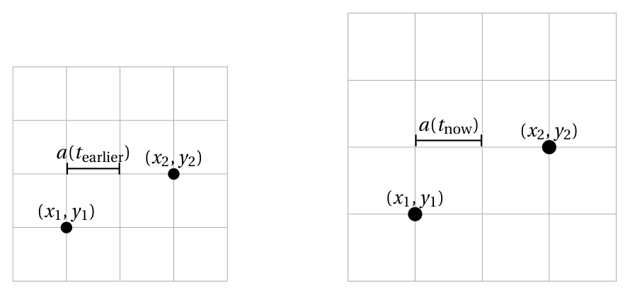
One way to understand the scale factor is to imagine a grid of points, as shown in Fig. 7.2.2. As time goes on the grid stretches. Not only does that increase the distance between the two indicated points, but it increases the distance between every possible pair of points. In that sense, \(a(t)\) represents the scale of the entire universe.

Figure \(\PageIndex{2}\): Two points are at fixed locations on a grid. As time passes, the grid stretches, which increases the distance between all possible pairs of points. (Copyright; author via source)

One interesting consequence of the fact that distances between two points change with time is that it is no longer true that light takes 1 year to reach us from an object that is 1 light-year away. To figure out the relationship between distance and time, let's look at the metric again. Suppose a distant light source emits light at \((r,t)=(r_\text{emit},t_\text{emit})\) and we receive that light at \((r,t)=(0,t_0)\). Because \(d\tau=0\) for light, the FLRW metric reduces to

\[\begin{align*}0&=dt^2-a^2(t)dr^2\\ dr^2&=\frac{dt^2}{a^2(t)}\\ dr&=\pm\frac{dt}{a(t)}\\ \int\limits_{r_\text{emit}}^0dr&=\pm\int\limits_{t_\text{emit}}^{t_0}\frac{dt}{a(t)}\\ -r_\text{emit}&=\pm\int\limits_{t_\text{emit}}^{t_0}\frac{dt}{a(t)}\end{align*}.\]

Therefore

\[r_\text{emit}=\pm\int\limits_{t_0}^{t_\text{emit}}\frac{dt}{a(t)}\label{eq:remit},\]

where we use whatever sign gives us a positive r-coordinate.

Exercise \(\PageIndex{3}\)

Observations indicate that the scale factor was zero approximately 14 billion years ago and that it has been monotonically increasing since then. It is also conventional to set \(a(t_0)=1\) (where the subscript of "0" represents "today"). Determine an expression for \(a(t)\) assuming that it has increased linearly.

Answer

We want a linear function (i.e. \(a(t)=mt+b\) )with \(a(0)=0\) and \(a(t_0)=1\). Substituting \(t=0\), we get \(a(0)=b\), which implies that \(b=0\). Substituting \(t=t_0\), we get \(a(t_0)=mt_0\), which implies that \(m=\frac{1}{t_0}\). Therefore \(a(t)=\frac{1}{t_0}t\).

Exercise \(\PageIndex{4}\)

A star emitted a beam of light 3 billion years ago and just now reaches us. What was the r-coordinate of that star at the moment it emitted the light? (Use the \(a(t)\) that you determined in the previous exercise.) What was the distance between us and the star when the light was emitted?

Answer

Eq.\ref{eq:remit} tells us how to determine the r-coordinate at which a beam of light was emitted given \(a(t)\) and the amount of time it took to reach us. We will set \(t_\text{emit}=11\text{ billion years}\) and \(t_0=14\text{ billion years}\).

\[\begin{align*}r_\text{emit}&=\pm\int\limits_{t_0}^{t_\text{emit}}\frac{dt}{\frac{1}{t_0}t}&&\\ &=\pm\int\limits_{t_0}^{t_\text{emit}}\frac{t_0\ dt}{t}&&\text{simplify}\\ &=\pm t_0\left [\ln t\right]_{t_0}^{t_\text{emit}}&&\text{evaluate integral}\\ &=\pm t_0\ln\left (\frac{t_\text{emit}}{t_0}\right)&&\text{substitute bounds}\\ &=\pm\left (14\text{ billion years}\right)\ln\left(\frac{11\text{ billion years}}{14\text{ billion years}}\right )&&\text{substitute numbers}\\ &=3.38\text{ billion light-years}&&\text{calculate}\end{align*}\]

At first this answer may seem confusing since, in an expanding universe, light emitted from 3.38 billion light-years away should take longer, not shorter, than 3.38 billion years to reach us. Remember, though, that being at an r-coordinate of 3.38 billion light-years doesn't mean that the star was 3.38 billion light-years away from us. For that we use Equation \ref{eq:FLRWProperDistance}.

\[\Delta \sigma = a\left(t_\text{emit}\right)r_\text{emit}=\left(\frac{11}{14}\right)\left (3.38\text{ billion light-years}\right)=2.65\text{ billion light-years}\nonumber\]

This answer makes sense. The time it takes for light to reach us from a star that used to be 2.65 billion light-years away from us is slightly longer than 2.65 billion years because the universe expanded in the meantime.