7.1: Modeling the Universe
- Page ID
- 46264
\( \newcommand{\vecs}[1]{\overset { \scriptstyle \rightharpoonup} {\mathbf{#1}} } \)
\( \newcommand{\vecd}[1]{\overset{-\!-\!\rightharpoonup}{\vphantom{a}\smash {#1}}} \)
\( \newcommand{\dsum}{\displaystyle\sum\limits} \)
\( \newcommand{\dint}{\displaystyle\int\limits} \)
\( \newcommand{\dlim}{\displaystyle\lim\limits} \)
\( \newcommand{\id}{\mathrm{id}}\) \( \newcommand{\Span}{\mathrm{span}}\)
( \newcommand{\kernel}{\mathrm{null}\,}\) \( \newcommand{\range}{\mathrm{range}\,}\)
\( \newcommand{\RealPart}{\mathrm{Re}}\) \( \newcommand{\ImaginaryPart}{\mathrm{Im}}\)
\( \newcommand{\Argument}{\mathrm{Arg}}\) \( \newcommand{\norm}[1]{\| #1 \|}\)
\( \newcommand{\inner}[2]{\langle #1, #2 \rangle}\)
\( \newcommand{\Span}{\mathrm{span}}\)
\( \newcommand{\id}{\mathrm{id}}\)
\( \newcommand{\Span}{\mathrm{span}}\)
\( \newcommand{\kernel}{\mathrm{null}\,}\)
\( \newcommand{\range}{\mathrm{range}\,}\)
\( \newcommand{\RealPart}{\mathrm{Re}}\)
\( \newcommand{\ImaginaryPart}{\mathrm{Im}}\)
\( \newcommand{\Argument}{\mathrm{Arg}}\)
\( \newcommand{\norm}[1]{\| #1 \|}\)
\( \newcommand{\inner}[2]{\langle #1, #2 \rangle}\)
\( \newcommand{\Span}{\mathrm{span}}\) \( \newcommand{\AA}{\unicode[.8,0]{x212B}}\)
\( \newcommand{\vectorA}[1]{\vec{#1}} % arrow\)
\( \newcommand{\vectorAt}[1]{\vec{\text{#1}}} % arrow\)
\( \newcommand{\vectorB}[1]{\overset { \scriptstyle \rightharpoonup} {\mathbf{#1}} } \)
\( \newcommand{\vectorC}[1]{\textbf{#1}} \)
\( \newcommand{\vectorD}[1]{\overrightarrow{#1}} \)
\( \newcommand{\vectorDt}[1]{\overrightarrow{\text{#1}}} \)
\( \newcommand{\vectE}[1]{\overset{-\!-\!\rightharpoonup}{\vphantom{a}\smash{\mathbf {#1}}}} \)
\( \newcommand{\vecs}[1]{\overset { \scriptstyle \rightharpoonup} {\mathbf{#1}} } \)
\(\newcommand{\longvect}{\overrightarrow}\)
\( \newcommand{\vecd}[1]{\overset{-\!-\!\rightharpoonup}{\vphantom{a}\smash {#1}}} \)
\(\newcommand{\avec}{\mathbf a}\) \(\newcommand{\bvec}{\mathbf b}\) \(\newcommand{\cvec}{\mathbf c}\) \(\newcommand{\dvec}{\mathbf d}\) \(\newcommand{\dtil}{\widetilde{\mathbf d}}\) \(\newcommand{\evec}{\mathbf e}\) \(\newcommand{\fvec}{\mathbf f}\) \(\newcommand{\nvec}{\mathbf n}\) \(\newcommand{\pvec}{\mathbf p}\) \(\newcommand{\qvec}{\mathbf q}\) \(\newcommand{\svec}{\mathbf s}\) \(\newcommand{\tvec}{\mathbf t}\) \(\newcommand{\uvec}{\mathbf u}\) \(\newcommand{\vvec}{\mathbf v}\) \(\newcommand{\wvec}{\mathbf w}\) \(\newcommand{\xvec}{\mathbf x}\) \(\newcommand{\yvec}{\mathbf y}\) \(\newcommand{\zvec}{\mathbf z}\) \(\newcommand{\rvec}{\mathbf r}\) \(\newcommand{\mvec}{\mathbf m}\) \(\newcommand{\zerovec}{\mathbf 0}\) \(\newcommand{\onevec}{\mathbf 1}\) \(\newcommand{\real}{\mathbb R}\) \(\newcommand{\twovec}[2]{\left[\begin{array}{r}#1 \\ #2 \end{array}\right]}\) \(\newcommand{\ctwovec}[2]{\left[\begin{array}{c}#1 \\ #2 \end{array}\right]}\) \(\newcommand{\threevec}[3]{\left[\begin{array}{r}#1 \\ #2 \\ #3 \end{array}\right]}\) \(\newcommand{\cthreevec}[3]{\left[\begin{array}{c}#1 \\ #2 \\ #3 \end{array}\right]}\) \(\newcommand{\fourvec}[4]{\left[\begin{array}{r}#1 \\ #2 \\ #3 \\ #4 \end{array}\right]}\) \(\newcommand{\cfourvec}[4]{\left[\begin{array}{c}#1 \\ #2 \\ #3 \\ #4 \end{array}\right]}\) \(\newcommand{\fivevec}[5]{\left[\begin{array}{r}#1 \\ #2 \\ #3 \\ #4 \\ #5 \\ \end{array}\right]}\) \(\newcommand{\cfivevec}[5]{\left[\begin{array}{c}#1 \\ #2 \\ #3 \\ #4 \\ #5 \\ \end{array}\right]}\) \(\newcommand{\mattwo}[4]{\left[\begin{array}{rr}#1 \amp #2 \\ #3 \amp #4 \\ \end{array}\right]}\) \(\newcommand{\laspan}[1]{\text{Span}\{#1\}}\) \(\newcommand{\bcal}{\cal B}\) \(\newcommand{\ccal}{\cal C}\) \(\newcommand{\scal}{\cal S}\) \(\newcommand{\wcal}{\cal W}\) \(\newcommand{\ecal}{\cal E}\) \(\newcommand{\coords}[2]{\left\{#1\right\}_{#2}}\) \(\newcommand{\gray}[1]{\color{gray}{#1}}\) \(\newcommand{\lgray}[1]{\color{lightgray}{#1}}\) \(\newcommand{\rank}{\operatorname{rank}}\) \(\newcommand{\row}{\text{Row}}\) \(\newcommand{\col}{\text{Col}}\) \(\renewcommand{\row}{\text{Row}}\) \(\newcommand{\nul}{\text{Nul}}\) \(\newcommand{\var}{\text{Var}}\) \(\newcommand{\corr}{\text{corr}}\) \(\newcommand{\len}[1]{\left|#1\right|}\) \(\newcommand{\bbar}{\overline{\bvec}}\) \(\newcommand{\bhat}{\widehat{\bvec}}\) \(\newcommand{\bperp}{\bvec^\perp}\) \(\newcommand{\xhat}{\widehat{\xvec}}\) \(\newcommand{\vhat}{\widehat{\vvec}}\) \(\newcommand{\uhat}{\widehat{\uvec}}\) \(\newcommand{\what}{\widehat{\wvec}}\) \(\newcommand{\Sighat}{\widehat{\Sigma}}\) \(\newcommand{\lt}{<}\) \(\newcommand{\gt}{>}\) \(\newcommand{\amp}{&}\) \(\definecolor{fillinmathshade}{gray}{0.9}\)In General Relativity, metrics come about by first proposing a matter/energy distribution and then solving the Einstein Field Equations. If we want to know the metric to apply to a star or black hole, for example, we can think of the universe as containing a single point mass with spherical symmetry. By imposing this constraint, we solve the Einstein Field Equations and discover the Schwarzschild metric.
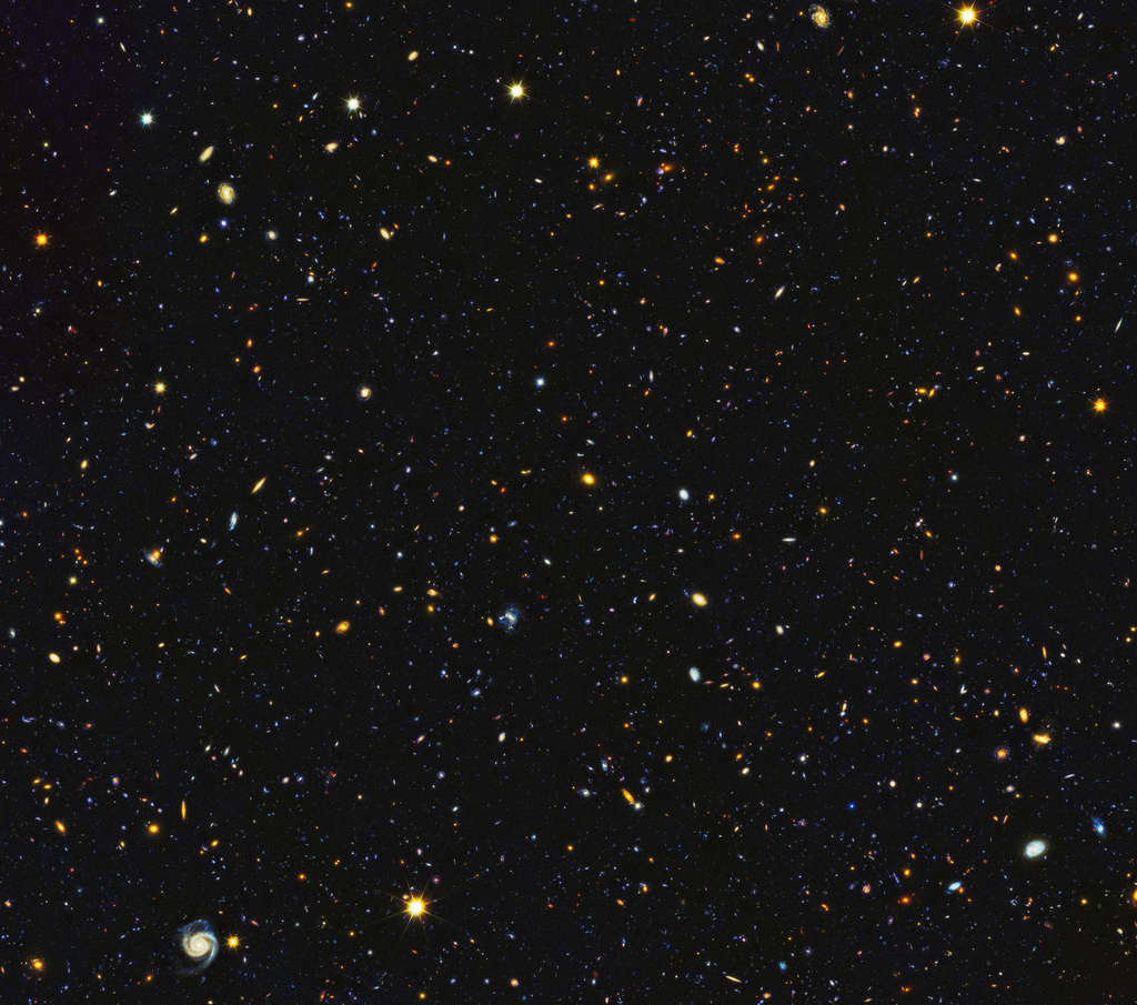
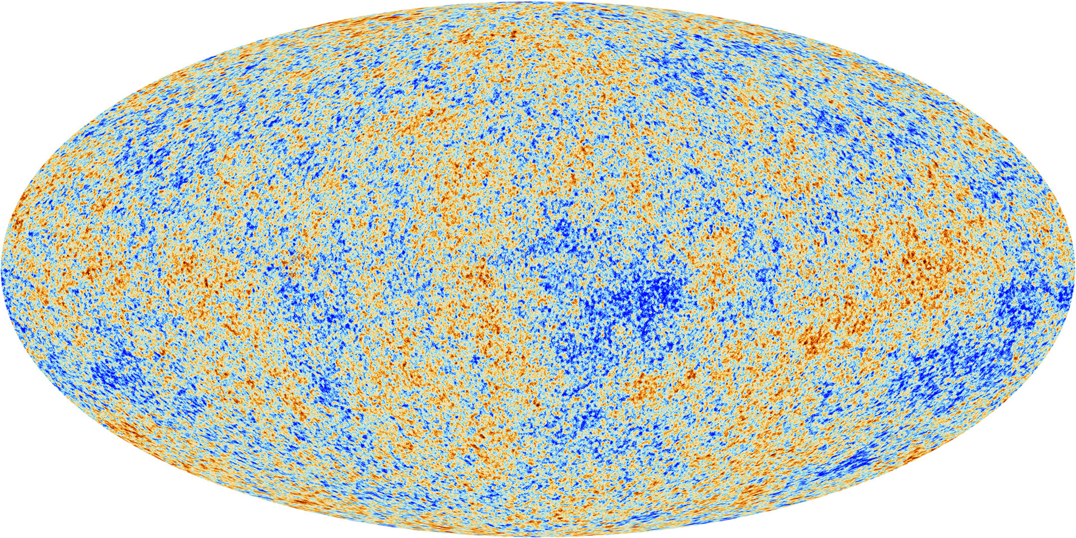
Suppose, however, that we want to determine a metric for the universe as a whole? What does the distribution of matter look like? What constraints can we impose? To answer that question, take a look at Figures \(\PageIndex{1}\) and \(\PageIndex{2}\). The former is an image of a portion of sky that is only 2.4 arc-minutes on each side yet contains approximately 10,000 galaxies. The latter is a temperature map of the early universe, where temperature roughly approximates matter distribution. The colors show variations relative to the mean of approximately \(10^{-5}\).


Based on Figs. 7.1.1 and 7.1.2, how would you describe the matter distribution of the universe?
- Answer
-
Both images show that matter is distributed roughly uniformly, as there is no obvious concentration in one location. Fig. 7.1.2 does show some "hotspots" and "coldspots" but the scale of those differences is incredibly tiny.
Figure \(\PageIndex{2}\) shows the concentration of matter in the early universe across the entire celestial sphere (that is, a sphere centered on earth). Because the variations from one location to another are so small, no matter what direction you look in you will see approximately the same concentration of matter. We say that the universe is isotropic from our perspective.
A system of particles is isotropic from a particular point of view if its properties are the same no matter what direction you look in.
The problem with isotropy is that it is very observer-centric. That is, it describes what things look like from one single point of view. If we want to describe the universe as a whole, then we also have to address the question of what things look like from the point of view of someone in the Andromeda galaxy, or any other galaxy for that matter. If everything does look the same from the point of view of someone in any other galaxy, then we say that the distribution of matter is homogeneous.
In a homogeneous system of particles, the properties of the system appear to be the same from all points of view.
Can you think of an example of something that is isotropic? Can you think of an example of something that is homogenous? Can you think of an example of something that is isotropic but not homogeneous? Homogeneous but not isotropic?
- Answer
-
One example of something that is isotropic is a Gobstopper, as shown in Figure \(\PageIndex{3}\). It is a hard candy that consists of many concentric spherical layers. It is isotropic as viewed from the center.

Figure \(\PageIndex{3}\): A Gobstopper is a hard candy that consists of spherical layers. (Image credit: Wikipedia) An example of something that is homogeneous is the surface of a pool cue ball. If you were to miniaturize yourself and stand on the surface, the surface would look the same to you no matter where you stood.
The Gobstopper is isotropic but not homogeneous because it does not look the same if you hopped to a location anywhere other than the center.
The pool cue ball is homogeneous but not isotropic because if you were standing on the surface and looked up versus looked down, you would see very different things.
Can a system of particles be homogeneous if it has edges?
- Answer
-
If a system of particles has edges, then you would see something different if you stood on one of the edges versus standing somewhere in the middle. Therefore anything with edges technically is not homogeneous. (Note that we are defining homogeneity different from how homogeneous mixtures are defined in chemistry, where mixtures can be homogeneous even if they are in a container.)
To be clear, while we can safely say that the universe appears to be approximately isotropic from our point of view, we can't necessarily say that it is homogeneous because we can't observe the universe from other locations. If the universe isn't homogeneous, though, then we can't make any claims about the matter distribution of the universe as a whole since the properties of the universe that we observe would just be due to the specialness of our own local patch. Therefore, we will assume that our local patch is not special in any way because we have no other option (or at least no option other than giving up). We call this the cosmological principle.
The cosmological principle is the assertion that the properties of the universe are the same for all observers when viewed on a large enough scale. This implies that the universe is isotropic and homogeneous.

