3.2: Intro Particle Model of Matter

Overview

In the Intro Particle Model of Matter we focus primarily on the interaction between two neutrally charged atoms or molecules. We make extensive use of the relation of force to potential energy in order to describe the force between two atomic sized particles. In the next two models will use the basic ideas established here to help us develop a much deeper understanding of both bond energy and thermal energy, as we will make the transition from the microscopic atomic level to the macroscopic perspective.

The Particle Model of Matter that we introduce here is the familiar picture of matter as composed of atoms and molecules. Our particle model for ordinary matter is simple and universal. It is not restricted to a particular kind of matter, but encompasses all ordinary matter. That is what makes this model so useful. Of course, being very general, it cannot predict many of the details that depend on the “particulars”, but it can predict many of the universal properties.

A Very Important Interaction

Repeating the quote by the famous Nobel laureate in physics, Richard P. Feynman:

"if, in some cataclysm, all of scientific knowledge were to be destroyed, and only one sentence passed on to the next generations of creatures, what statement would contain the most information in the fewest words? I believe it is the atomic hypothesis (or the atomic fact, or whatever you wish to call it) that all things are made of atoms—little particles that move around in perpetual motion, attracting each other when they are a little distance apart, but repelling upon being squeezed into one another. In that one sentence, you will see, there is an enormous amount of information about the world, if just a little imagination and thinking are applied.” -The Feynman Lectures on Physics, Volume I, page 1.

We will now go on to represent the words highlighted in red in terms of a potential energy between two subatomic particles.

Lennard-Jones Potential

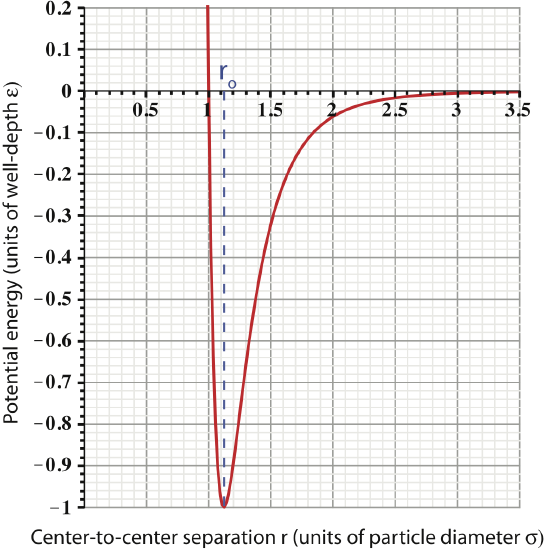
We will spend the rest of this section understanding the meaning of Feynman's statement. Graphically, the key points in Feynman's statement that describe the way neutral particles interact are represented in the figure below which we will set out to understand. The relationship illustrated in the figure was developed by John Lennard Jones in 1924, known as the Lennard-Jones potential (sometimes abbreviated as the LJ potential). More generally, this is known as the pair-wise potential, since it describes an interaction between a pair of particles.

Figure 3.3.1: Pair-wise Potential between neutrally charged subatomic particles (modeled by the Lennard-Jones potential).

Let us define some important characteristics seen in this plot:

• Particle: we use the general word "particle" to refer to a microscopic constituent of matter, since the Lennard-Jones potential models interactions between either neutral atoms or neutral molecules.
• Center-to-center separation: we consistently refer to the distance between particles as being the center-to-center separation, rather than the distance between their surfaces. Usually we will use the symbol r to indicate this separation distance.
• Particle diameter: is the diameter for a particular atom or molecule, for which we use the symbol \(\sigma\). It is useful to represent the particle seperation r in units of diameter, since this allows a universal scale. However, if the particle separation was shown in terms of units of length instead, such as nanometers (1nm=10^-9m), the plot would provide more information about the types of atoms or molecules that are interacting.
• Equilibrium separation: there is a “special” separation for which we use the symbol r_o. This separation is "special" since it is when the inter-particle force is zero. Looking at the figure above, we see that the slope of the PE plot goes to zero at \(r=r_o\), which tells us force is zero (recall the discussion in Section 2.7). In terms of particle diameter, \(r_o=1.12\sigma\), an important fact that you should commit to memory.
• Well-depth: the value of the potential energy at the equilibrium separation is know as the well-depth of the LJ potential, symbolically represented by \(\varepsilon\). This is the value of the minimum potential energy, \(PE_{LJ}(r=r_o)=-\varepsilon\). The units of \(\varepsilon\) are joules, since potential energy must have units of energy.

Algebraically the Lennard-Jones potential is written as:

\[PE_{LJ}(r)=4\varepsilon\Big [\Big(\frac{\sigma}{r}\Big)^{12}-\Big(\frac{\sigma}{r}\Big)^6 \Big] \]

Although, the subscripts "12" and "6" may seem strange, this form of the potential most accurately represent neutral interacting subatomic particles. If you plug this equation into a graphic calculator, you should find a shape seen in Figure 3.3.1.

Forces Between Neutral Particles

Let us return to the relationship between force and potential energy developed in Section 2.7 in order to help us understand the forces involved between particles whose interaction is described by the Lennard-Jones potential. Since the LJ potential is described in terms of particles separation r, it is useful to rewrite the force-potential energy relationship as:

\[ F_r = -\frac{dPE}{dr} \label{force.PE}\]

Atomic sized particles exert forces on each other in the same way that large-scale objects do. These forces can be attractive or repulsive. The Lennard-Jones potential has similarities to the spring-mass system. A mass hanging on a spring hangs at a particular “separation” from the point at which the spring is supported. This is the favored or the equilibrium position. If the mass finds itself closer to the point of support, the “spring force” pushes it away, back toward the equilibrium position. Conversely, if it finds itself too far form the support, the spring force pulls it back toward the equilibrium position. The exact same thing happens with two atomic sized particles. However, unlike the spring-mass potential which is parabolic, the LJ potential only appear to be parabolic near equilibrium separation r_o, but becomes steeper for values less than r_o and flattens out for values larger than r_o.

Feynman's statement claims that for small separations, \(r<r_o\), the force is repulsive: "repelling upon being squeezed into one another". The force relationship in Equation \ref{force.PE} states that when the slope of the PE plot is negative (as in the \(r<r_o\) region), the force, \(F_r\) will be positive, which means it points in the direction of positive or increasing particle separation, r. In other words, the force points in the direction that increases separation pushing the particles apart as they are squeezed together, thus the force is repulsive, as Feynman claims.

Another part of Feynman's statement states that for slightly larger separations the force becomes attractive,"attracting each other when they are a little distance apart". In the region for separations slightly larger than equilibrium, \(r>r_o\), the slope in Figure 3.3.1 becomes positive, thus the the force becomes negative. This means that the force points toward the -r direction, or toward decreasing particle separation, implying the force is pulling the particles together or is attractive.

We also observe that as the particle separation gets larger, \(r \gtrsim 3\sigma\), the slope of the PE plot goes to zero, thus, the force goes to zero as well. Since the force goes to zero at rather small separations (only 3 diameters apart!), this pair-wise interaction is known as short-range.

The figure below summarizes the forces between particles for different values of separation.

Figure 3.3.2: Forces between two neutral particles.

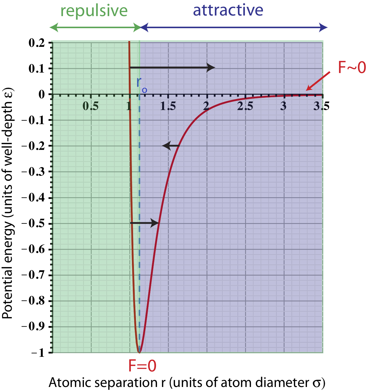
There are two force arrows drawn on the plot that represent repulsive (pointing to the right toward larger r's) forces at different values of separation. At very small values of r, the force is larger (longer arrow) since the slope of the plots gets steeper (Equation \ref{force.PE} tells us that the magnitude of force increases with the magnitude of the slope). This short distance repulsion tells us that particles cannot overlap or be squeezed into each other. The deeper explanation of this behavior is quantum mechanical and comes from the Pauli-exclusion principle, which we will not cover in this course. As the separation gets slightly bigger, the slope decreases, so the force becomes less repulsive, as shown by a shorter arrow on the graph. (Note, the relative arrow lengths are not drawn to scale.) A force arrow pointing to the left (shorter than the other two due to smaller slope) is shown to represent a separation when the force is attractive.

The fact that the force goes from being repulsive at small distances to attractive at large ones, implies that there is some particular separation which particles seem to prefer. Mathematically, in order for the slope of any plot to go from negative to positive, the potential energy must have an extremum point, such as a minimum or a maximum. This is represented by the potential minimum at the equilibrium separation \(r_o\), where the slope, and thus the force, goes to zero, as marked on the plot.

Alert

As seen on the plot the Lennard-Jones potential energy is zero at a separation of one diameter. It is tempting to assign some importance to this separation since the potential energy goes from being positive to negative as the particles move further apart. However, the physical characteristics of the interacting system is described by the slopes of the potential energy, giving us the directions and magnitudes of forces at different separations. In other words, if we shifted the entire plot up, it would still describe the same type of interaction since the slopes would not change. But shifting the plot upward would change where the graph crosses the x-axis. Thus, this location happens to have zero potential energy only due to the convention of choosing the potential energy to go to zero at far separations, and has no physical significance. This is similar to choosing the origin in order to define the "zero" of gravitational potential energy.

Bound and Unbound States

So far we have discussed the pair-wise potential energy between two interacting neutral particles. We also noted that the behavior of particles interacting with the LJ potential is very similar to the spring-mass system, at least for separation close to equilibrium, which does appear parabolic (like PE_sm) near r_o. When the spring-mass system is displaced from equilibrium and released, it starts to oscillate speeding up at equilibrium, slowing down, and then stopping at the points of maximum displacement before turning around. Thus, the spring-mass transfers its energy between potential and kinetic while keeping the total energy constant, as long as friction is negligable. Similar ideas can be applied to two particles interacting with the LJ potential.

Picture a two-particles motionless and at their equilibrium separation. There are no forces acting on the particles, thus they will remain motionless with zero kinetic energy. At \(r_o\): \(E_{tot}=PE+KE=PE(r_o)=-\varepsilon\). This is analogous to a spring-mass system at rest and at its equilibrium position. What happens when energy is added to the two-particle system? In the spring-mass system we add energy as work by stretching (or compressing) a spring. Analogously, energy can be added to the two-particle system by pulling the particles apart or pushing them together away from their equilibrium separation.

We know that for the spring the end result is oscillating behavior. Let us look at an example of adding \(0.5\varepsilon\) of energy to the two-particle system. Since the initial energy at equilibrium was \(-\varepsilon\), adding this amount of energy results in \(E_{tot}=-0.5\varepsilon\). This total energy is plotted in the figure below.

Figure 3.3.3: Total Energy representing bound particles.

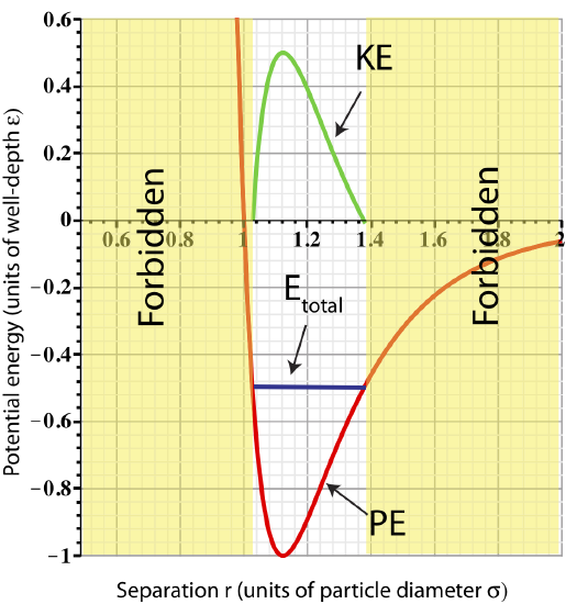
The figure shows us that adding \(0.5\varepsilon\) of energy is equivalent of separating the two particles from \(r_o\) to \(~1.4r_o\) or squeezing them to \(~1.03r_o\) (look at the values of r where E_total intercepts PE). Let us assume the particles where pushed apart to \(~1.4r_o\) and "released". At this separation the particles experience an attractive force pushing them back to equilibrium. (Equivalently, when a spring-mass is stretched, the restoring force points back to equilibrium.) As the particles return to equilibrium, their potential energy will decrease, while kinetic energy increases. Since PE_LJ is minimum at r_o, the particles will be moving the fastest at this separation. As they move past equilibrium to separations smaller than r_o, they will start feeling a repulsive force and will gain PE and loose KE. Kinetic energy will go to zero at the minimum separation, \(r_{min}\sim 1.03r_o\), at which point the particles will start moving apart. This behavior will continue in this oscillatory manner (as for the spring-mass) as long as there is no source of energy loss. The plot for KE as a function of particle separation is shown in Figure 3.3.3.

Any separation smaller than r_min is not allowed (marked "forbidden" on the plot). At the minimum separation the total energy equals to the potential energy. At separations smaller then r_min the potential becomes greater than the E_tot. In order to obey conservation of energy, \(E_{tot}=PE_{LJ}+KE\), that would imply that \(KE<0\) when \(r<r_{min}\), since \(PE_{LJ}>E_{tot}\). Kinetic energy cannot be negative since it is proportional to speed squared, \(KE=\frac{1}{2}mv^2\). Thus, having a separation smaller than r_min is not physical, and thus, forbidden. Using the same arguments, any separation larger than r_max results is \(KE<0\), and therefore, is forbidden.

When the particles oscillate back and forth about their equilibrium separation, we call them bound to each other, since they cannot move independently of each other. As we add more energy to the system, the E_tot line will move up and the distance between r_min and r_max will increase, thus the particles will oscillates with a greater ranges and a faster speed at equilibrium.

A summary of bound particle characteristics:

• Total energy: \(E_{tot}=PE_{LJ}+KE\). For the particle to be bound \(E_{tot}<0\).
• Minimum separation: \(r_{min}\) is the smallest allowed separation for a given value of \(E_{tot}\).
• Maximum separation: \(r_{max}\) is the largest allowed separation for a given value of \(E_{tot}\).

As the total energy approaches zero, the total energy plot no longer intersects the potential energy on the right. Let us look at an example of \(E_{tot}=0.5\varepsilon\) as shown in the figure below. In this case, since \(E_{tot}>PE\) for separations of \(r>r_{min}\), kinetic energy will always stay positive at these separations. This implies that the two particles will move apart at large separations where they are no longer interacting since the force goes to zero for \(r \gtrsim 3\sigma\). Once the two particles are far apart, there is no force acting to bring them back together. They become independent of each other, and, thus, we call them unbound.

Figure 3.3.4: Total Energy representing unbound particles.

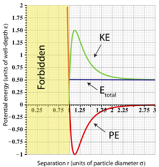
A summary of unbound particle characteristics:

• Total energy: \(E_{tot}=PE_{LJ}+KE\). For the particle to be unbound \(E_{tot}\geq 0\).
• Minimum separation: \(r_{min}\) is the smallest allowed separation for a given value of \(E_{tot}\).
• Maximum separation: the is no limit on maximum separation since \(KE\geq 0\) for all values of \(r\geq r_{min}\).

Example \(\PageIndex{1}\)

UC Davis scientists discover two new atoms, Aggieum (Ai) and Cyclerium (Cy). The plot below shows Lennard-Jones potential energies for Ai-Ai and Cy-Cy atoms.

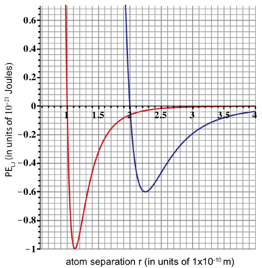
a) The diameter of Cy is twice the diameter of Ai. Determine the diameter of both from the given plot. Label the two curves as either Ai-Ai or Cy-Cy potential energy.

b) A pair of atoms is oscillating with a \(E_{tot} = -0.6\times 10^{-21}\) Joules. Determine which pair (Ai-Ai or Cy-Cy) is oscillating and plot the corresponding E_tot and KE.

c) For the result in b), is the pair bound or unbound? If bound, how much more energy do you need to add in order to break the bond between the two atoms.

Solution

a) Diameter of Ai is 1x10^-10 m, and diameter of Cy is 2x10^-10m. Atom diameter is found from the Lennard-Jones potential when PE intercepts the x-axis.

b) Only the Ai-Ai pair will be oscillating with \(E_{tot} = -0.6\times 10^{-21}\) Joules. Cy-Cy pair at this energy will be stationary and at equilibrium (E_tot intercepts PE at one point). We obtain the plot for KE as shown in the figure below, by using E_tot = KE + PE. E_tot is constant due to conservation of energy.

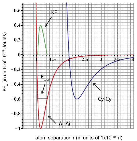
c) When \(E_{tot} = -0.6\times 10^{-21}\) Joules the atoms oscillate between r_min and r_max as shown in the plot, thus they are bound. You need to add \(0.6\times 10^{-21}\) joules of energy to reach E_tot=0, at which point the atoms become unbound.

From Two to Many Particles

When there are many particles, the phase (solid, liquid, or gas) of those particles depends on their total energy. At sufficiently high total energy, the particles are unbound and in the gas phase. At sufficiently low energy the particles are in the liquid or solid phase and are bound. The average particle-particle separation in the bound state is approximately equal to the separation corresponding to the minimum of the pair-wise potential energy. In the unbound state it is much greater than the separation corresponding to the minimum PE.

The macroscopic size of matter, whether it is in a solid, liquid or gas phase, is due to the simultaneous interactions of something like ~10²³ pair-wise interactions if we have a mole of the substance. Our task in the next two sections will be to go from the two-particle microscopic description summarized in this section to the macroscopic sizes of matter. These ideas are far from simple. Initially, try to imagine a solid at very low temperatures (KE is nearly zero). Each particle “wants” to be at the right distance with respect to all of its neighbors. If there is a way for the system to “get rid” of its energy (by giving it to some colder system, for example), it will continue to settle down and reduce its thermal energy. Eventually, all the random motion comes to a stop (if we can keep cooling the sample) and the particles find their “magic” places, each near the “bottom” of the PE_pair-wise with each of their neighbors.

Now, imagine we start adding energy to the sample. All the particles begin acting like little spring-masses, oscillating back and forth around their equilibrium positions. Eventually they move sufficiently far, so that some “jump” out of where they are “supposed to be". Particles at or near the surface might even leave the sample if their vibrations get vigorous enough. Picturing what happens when a substance melts, i.e., turns from a solid to a liquid, is difficult, even for the experts. Don’t worry about picturing that transition. But you can imagine continuing to add energy until all the particles, even 10²³ particles, have sufficient energy to separate far apart from each other, causing them to be in the gas phase. So, what is the bottom line here at this point in our making sense of all this? Without getting into a lot of detail, it should make sense to you that at some sufficiently low temperature, everything will be a solid and at some sufficiently high temperature, everything should be a gas. That is plenty for right now.