5.8: Exponential Change Model

We have dealt mainly with steady-state conditions in the discussion up to this point. Among other things, this means that the gradient of the potential remains constant in time. This will typically be the case when there is a large reservoir of whatever it is that is being transported on both sides of the region through which the transport is occurring. Then, if the reservoirs remain at constant potential, one higher than the other, the potential gradient remains constant resulting in a constant flow rate. For example, heat will flow from a building kept at a fixed temperature, by an air conditioner, to the outside environment whose temperature is also fixed. Since the difference between the temperatures of the inside and outside remains the same, the rate of heat flow will be constant and the system will remain in a steady-state. 

In more general cases, the potential (and the potential gradient) is a function of both time and spatial dimensions. We know that a cold drink will eventually warm up when left outside on hot day, so the potential gradient, i.e. the temperature difference between the drink and the outside will change with time, resulting in a non steady-state flow rate or power. By combining the transport equation with the condition of continuity and conservation of energy-density, a differential equation is obtained which will result in an exponential change of flow rate.

Exponential Decay

Before we go into physical examples that demonstrate exponential change, we will describe the mathematics of the exponential function. Things grow (or decay) exponentially when the time rate of change in a quantity is proportional to the amount already present. Bacteria grow exponentially because the more you have, the more they reproduce (until they run out of food, or their waste starts to poison the environment). The decay of radioactive elements is exponential because as the number of radioactive atoms decreases, there are fewer available to decay, so less decay occurs. The key idea is that the rate of change depends on the amount present. Mathematically, the previous statement it looks like this:

\[\dfrac{dy}{dt} = \pm\lambda y\label{exp}\]

In words the above equation states that the rate of change in \(y\) is proportional to \(y\) , and the constant of proportionality is \(\lambda\). If the sign in front of \(\lambda\) is positive, then \(y\) is getting bigger (e.g., growth of organisms or compound interest). If the sign is negative, then \(y\) is getting smaller (e.g., decay of voltage across a cell membrane or nuclear decay.) Again, this is the key to having exponential change. The rate of change is proportional to the amount present at that time. There is only one function which results in itself with you take it derivative, and it is an exponential: \(\dfrac{d}{dx}e^x=e^x\). In this section we will focus on things that decay exponential, thus we will only see a negative sign in the exponent for exponential decay phenomena. 

Solving Equation \ref{exp} for \(y(t)\) required some calculus. We will focus on the importance of the result and interpretation of exponential decay phenomena. Thus, you can skip directly to the result shown below in Equation \ref{exp-result} below. But if you are interested in seeing the mathematics of obtaining the result, you can read through the "derivation" box shown below.

Derivation

We start with equation for general exponential decay:

\(\dfrac{dy}{dt} = -\lambda y\)

The equation above can be rearranged such as the y-dependent terms are on one side and the time term is on the other side: 

\(\dfrac{dy}{y} = -\lambda dt\)

Now we can take the integral of each side of the equation and integrate from initial time, \(t=0\), to same later time \(t^{\prime}\).  Let us define the value of \(y\) at \(t=0\) to be \(y_0\).  So we integrate \(y\) from \(y_0\) to some arbitrary value \(y^{\prime}\).  The "prime" is there to distinguish \(t^{\prime}\) from \(t\) and \(y^{\prime}\) from \(y\). Integrating both sides we get:

\(\int_{y_0}^{y^{\prime}}\frac{dy}{y} = -\int_{0}^{t^{\prime}}\lambda dt\)

This results in:

\(\ln(y^{\prime}) - \ln(y_0) = -\lambda t^{\prime}\)

Using the property of log, \(\ln\Big(\dfrac{a}{b}\Big)\equiv\ln(a)-\ln(b)\), we get:

\(\ln\Big(\dfrac{y}{y_0}\Big)=-\lambda t\)

Using the following property that related the exponential with the natural log:

\(e^{\ln(x)}=x\),

and taking the exponential of each side of the equation and dropping the "prime", we get:

\(\dfrac{y}{y_0}=e^{-\lambda t}\).

Finally solving to \(y\) gives us the expression of how \(y\) changes as a function of time:

\(y(t)=y_0e^{-\lambda t}\)

When solving the differential equation \ref{exp} as outlined in the derivation above we arrive at the following expression for the time dependence of the variable \(y\):

\[y(t)=y_0e^{-\lambda t}\label{exp-result}\]

Whenever you get a result like this with an exponential function it is always helpful to calculate the extreme values, in other words, the value of y at \(t=0\) and at \(t\gg 0\) to figure out the value which the variable approaches in the case of exponential decay. Using the exponential property, \(e^0=1\) and evaluating Equation \ref{exp-result} at \(t=0\) we conclude that \(y(t=0)=y_0\). This is exactly the definition of \(y_0\), the value of \(y\) at \(t=0\) (see Derivation). To find the value of \(y\) when \(t\gg 0\) we can take the limit of \(y(t)\) when \(t\) goes to infinity.  Using the following property, \(\lim_{x \to \infty}e^{-x}=0\), we find that \(y\) decays to zero. A plot of \(y\) as a function of \(t\) is shown below.

Figure 5.8.1: Function Demonstrating Exponential Decay.

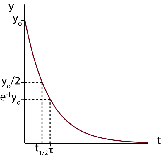
Another question we want to address is how fast the decay occurs. A very useful way to measure the rate of this decay is by using a concept of half-life. Half-life, \(t_{1/2}\) tells us how long it takes for an amount which is changing exponentially to get to the value which is halfway between the original value at \(t=0\) and the final equilibrium value at \(t\gg 0\). Half-life has units of time, such as seconds, minutes, hours, or years. The definition of half-life is depicted in Figure 5.8.1 above, the time at which when the amount \(y\) has reached a value of \(y_0/2\).

Alert

It does not necessarily mean that it took one half-life for the amount to get to half of its original amount, since the final equilibrium value does not have to be zero for exponential decay to occur. For example, if the system starts at a value of 10 and goes to 0, then indeed half-life will mean the time it takes for the amount to get to half of the original value of 10, i.e. 5.  However, if the system starts at a value of 10 but approaches 2 as its equilibrium final value, then half-life will be the time it takes for the system to get to 6, which is the amount halfway between 10 and 2. 

Now let us see how to calculate half-life from Equation \ref{exp-result}. Since in this case \(y\) decays to zero in this case, half-life, \(t_{1/2}\), is the time when \(y\) reaches half of its original value, \(y(t_{1/2})=\dfrac{y_0}{2}\). Plugging this into Equation \ref{exp-result} we find that:

\[y(t=t_{1/2})=\dfrac{y_0}{2}=y_0e^{-\lambda t_{1/2}}\]

Cancelling \(y_0\) from both sides of the equation and taking the natural log of both sides we get:

\(\ln\Big(\dfrac{1}{2}\Big)=-\lambda t_{1/2}\)

Finally, using the natural log property, \(\ln\Big(\dfrac{1}{x}\Big)=-\ln(x)\) we find that:

\[t_{1/2}=\dfrac{\ln 2}{\lambda}\label{half-life}\]

The above equation tells us that the larger the value of \(\lambda\) the smaller will be the half-life, the faster the decay and vice versa. (Try plotting the exponential Equation \ref{exp-result} for different values of \(\lambda\) and observe how it effects the decay rate). Half-life can be easily estimated if you have data or a plot the exponential decay. Another useful measure of decay rate is the time constant, which also has units of time and can readily obtained if you know the value of \(\lambda\).  By definition time constant, \(\tau\), is the inverse of \(\lambda\):

\[\tau\equiv\dfrac{1}{\lambda}\label{tau}\]

To find the value of \(y\) when \(t=\tau\) we can plug the definition of \(\tau\) into Equation \ref{exp-result}:

\[y(t=\tau)=y_0e^{-\lambda\tau}=y_0e^{-1}\sim 0.368y_0\]

The value of \(\tau\) is depicted in Figure 5.8.1. The time constant is slightly larger than half-life since it is the time it take for the system to get to \(0.368y_0\) of its original value which is less than \(0.5y_0\) for half-life. So the system has to decay for a longer time to get to a smaller amount. Half-time and time constant can be related to each other by using Equations \ref{half-life} and \ref{tau}:

\[t_{1/2}=\dfrac{\ln 2}{\lambda}=\tau\ln 2\label{tau-half}\]

Example \(\PageIndex{1}\)

A radioactive material decays exponentially from its initial amount of \(N_0\). It take the material 15 years to get to \(75\%\) of its initial amount. Find the half life of this material.

Solution

For radioactive decay:

\(N=N_0e^{-\lambda t}\) 

It takes 15 years to get to \(75\%\) of \(N_0\), such that \(N(t=15~\text{years})=\dfrac{3}{4}N_0\):

 

\(y(t=15)=\dfrac{3}{4}N_0=N_0e^{-15\lambda}\)

resulting in,

\(\dfrac{3}{4}=e^{-15\lambda}\)

Taking the natural log of both sides:

\(\ln\Big(\dfrac{3}{4}\Big)=-15\lambda\)

Using \(\ln\dfrac{1}{x}=-\ln x\) and solving for \(\lambda\):

\(\lambda=\dfrac{\ln\Big(\dfrac{4}{3}\Big)}{15}=0.01918~\dfrac{1}{\text{years}}\)

We can find half-life using Equation \ref{tau-half}:

\(t_{1/2}=\dfrac{\ln 2}{\lambda}=\dfrac{\ln 2}{0.01918}= 36.1~\text{years}\)

We now have introduced all the important components of exponential decay and are ready to apply them to real physical situations.