5.9: Exponential Fluid Flow

A Leaking Container

The scenario shown below in Figure 5.9.1 is a cylinder that is initially filled with a liquid. There is an opening toward the bottom of the container which is initially closed with a valve. When the valve is open at some later time, the liquid becomes exposed to the atmosphere and starts to leak out of the container. The rate at which the fluid is flowing, the current, depends on the total head gradient between the bottom and the top of the container. We will assume that there is an overall resistance to the flow. Once the valve is open the pressure difference between locations 1 and 2 is zero since both are at atmospheric pressure. The gravitation potential energy-density gradient is not zero, on the other hand, and is proportional to the height of the fluid inside the container. However, this height decreases as the liquid flows out of the cylinder, resulting in a decrease of current. Thus, we have an example of a fluid flow system where the flow is no longer steady-state. In fact, the current, which is rate of change of volume, is proportional to the amount of volume present. This is exactly how we described a system which behaves exponentially in Section 5.8.  

Figure 5.9.1: Non Steady-State Fluid System: leaking container

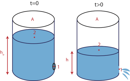
When the valve is open to the atmosphere the pressure difference between points 1 and 2 is zero, but there is a change in gravitational potential energy-density. Applying Bernoulli equation between these two points in the direction of current we get:

\[-\rho gh=-IR\label{cylinder-leak}\]

This equation may seem very familiar from examples in previous sections, but the current is no longer a constant here, since height, \(h\), depends on time. At t=0 the height is \(h_0\) resulting in an initial current \(I_0\) of:

\[I_0=\dfrac{\rho gh_0}{R}\label{I0}\]

Current is the rate of change of volume. In the Bernoulli equation current must be a positive quantity in order for the \("-IR"\) term to be negative to represent a loss of mechanical energy to thermal energy. In this case volume is decreasing as a function of time, so the quantity \(\dfrac{dV}{dt}\) is negative, thus the negative sign needs to be added in order to make the current positive:

\[I=-\dfrac{dV}{dt}\label{It1}\]

We can represent height in terms of volume by using \(V=Ah\), where \(A\) is the area of the cylinder as shown in Figure 5.9.1. Plugging in Equation \ref{It1} into Equation \ref{cylinder-leak} and solving for the rate of change of volume we arrive at:

\[\dfrac{dV}{dt}=-\dfrac{\rho g}{AR}V\label{Vt}\]

If you refer back to Section 5.8 you will see that the equation above has the exact form as the equation in the derivation of exponential decay, where \(\lambda=\dfrac{\rho g}{AR}\).  Using the result from the derivation we find that height changes with time as:

\[V(t)=V_0\exp\Big({-\dfrac{\rho g}{AR}t}\Big),\]

where \(\exp(x)\equiv e^x\) and \(V_0=Ah_0\). Using the Equation \ref{It1} we can solve for current by taking the derivative of Equation \ref{ht} and multiplying by a minus sign:

\[I(t)=\dfrac{\rho gh_0}{R}\exp\Big({-\dfrac{\rho g}{AR}t}\Big)=I_0\exp\Big({-\dfrac{\rho g}{AR}t}\Big)\]

We see that we get the exact value of initial current we found in Equation \ref{I0}. The current and the volume both decay exponentially to zero. 

Leaking Between Two Containers

Let us look at another similar but slightly modified situation shown below in Figure 5.9.2. Here there are two cylinder connected by a thin pipe. We start with all the fluid in the left cylinder held in place by a closed valve. Once the valve is open the liquid is allowed to flow. The current is determined by the pressure gradient between points 1 and 2 which is proportional to the height difference of the liquid in the two containers. As more fluid flows to the right cylinder the pressure difference decreases, and so does the current. Eventually the system approaches equilibrium when the water levels in the cylinders approach the same value resulting in equal pressures and zero current.

Figure 5.9.2: Non Steady-State Fluid System: two cylinder system

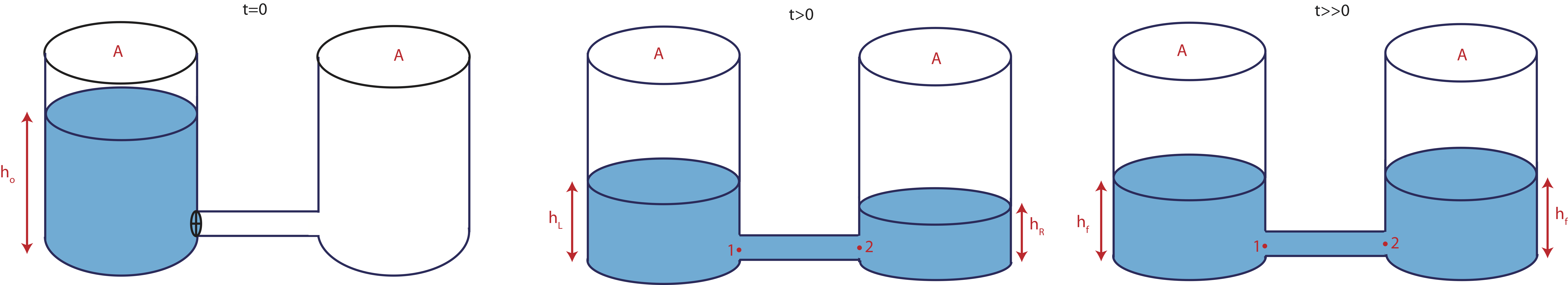
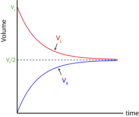
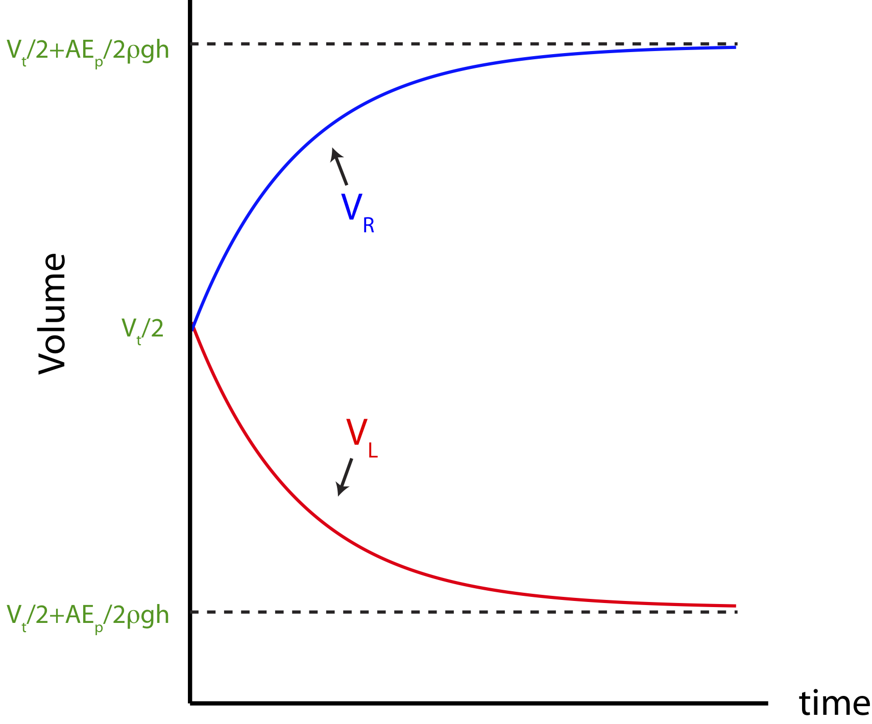
Since rate of charge of volume is proportional to the volume that is present, which means that the behavior will be exponential once again. You can arrive at these conclusions without doing all the math that we previously showed. Here we see an example where the quantity decaying exponential does not approach zero. The volume in the right cylinder starts at zero and approaches half the total volume exponentially. In the left cylinder the volume starts at the total volume and approaches half the total volume, again exponentially with the same rate. The volume in both cylinders displays exponential decay, even though the volume is increasing in one cylinder and decreasing in the other. The plots for volume as a function of time are shown in Figure 5.9.3 below.

Alert

Exponential decay does not mean that the value decreases from some initial value to zero or a smaller value. The word "exponential decay" implies that the parameter approaches another value in an exponential way.  That values can be larger than its initial values. 

Figure 5.9.3: Volume as a function of time: two cylinder system

You can follow the following basics procedures to conceptually arrive at the exponential change of the system without going through all the mathematics:

1. Establish that the system will change exponentially by arguing that the rate of change of some parameter is proportion to the value of that parameter.
2. Determine the value of the parameter at initial time.
3. Determine the value parameter as the system approaches steady-state or equilibrium.
4. Connect the initial and final values with an exponential function using any information you have about decay rate, such as time constant or half-life.

A Pump Moving Liquid Between Two Containers

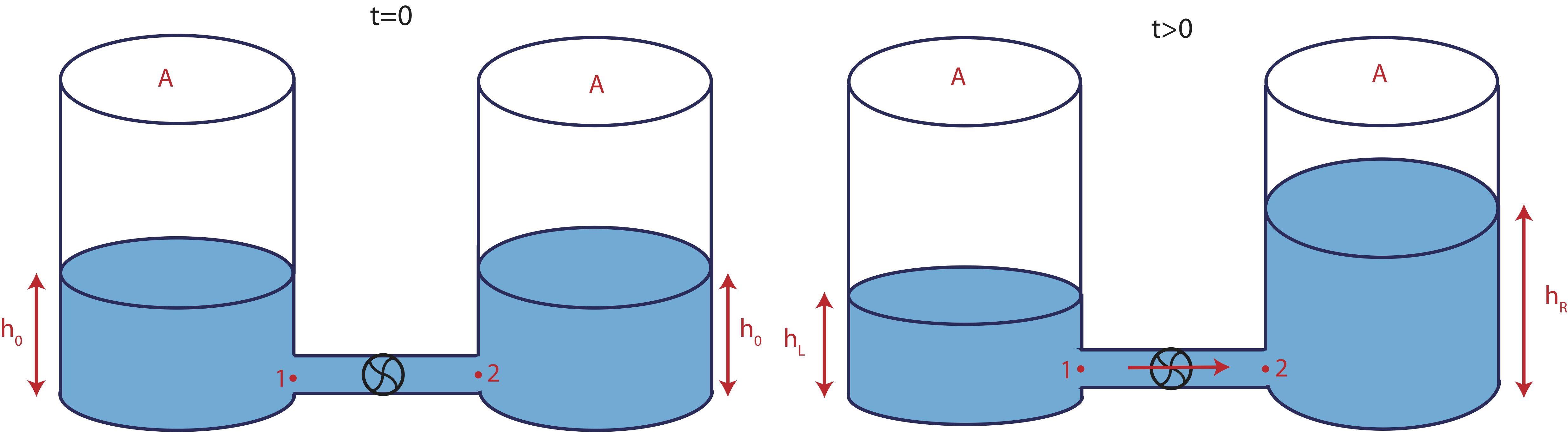
Imagine another example depicted below in Figure 5.9.4. There are two cylinders that initially contain the same amount of water. Thus, the heights of the water levels in each cylinder are equal. This mean that the pressures at points marked 1 and 2 are equal as well. The pump shown in the figure is initially turned off. There is no other source of potential gradient, the change in total head between points 1 and 2 is zero, resulting in zero current at t=0. Suddenly, the pump is turned on pumping fluid to the right, which results in more fluid accumulating in the right cylinder and fluid draining from the left cylinder. There is now a pressure gradient between points 1 and 2, resulting in a current which is proportional to this pressure difference. However, as the relative water level continue to change, so does the pressure gradient, resulting in a changing non steady-state current.

Figure 5.9.4: Non Steady-State Fluid System: filling up a container with a pump

We can use similar reasoning described above in red to figure out how the current and the volume change as a function of time. But we do require slightly more mathematical thinking here to found out the initial value of current, the final height and volume in each cylinder, and the decay rate.  We will do through this exercise here. Initially, at t=0, the instant the pump is turned on and water starts to flow to the right. We can assume that the instant the pump is turned on the water levels are still equal, resulting in \(\Delta(\text{total head})=0\) between points 1 and 2.  The complete Bernoulli equation at t=0 becomes:

\[0=\tilde{E}_{\text{pump}}-I_0R,\]

where we defined \(\tilde{E}_{\text{pump}}\equiv\dfrac{E_{\text{pump}}}{V}\) for simplicity. Solving for current we find:

\[I_0=\dfrac{\tilde{E}_{\text{pump}}}{R}\label{I-t0}\]

At some time later as the pump continues to work at constant strength, the two heights are no longer equal as shown in Figure 5.9.4 at \(t>0\). Assuming both cylinders are open to the atmosphere, the pressures at points 1 and 2 are given by:

\[\text{point 1:   }P_1=P_{atm}+\rho g h_L\]

\[\text{point 2:   }P_2=P_{atm}+\rho g h_R\]

Subtracting the two equations we can find the pressure difference between the two points and write down the Bernoulli equation between points 1 and 2:

\[P_2-P_1=\rho g (h_R-h_L)=\tilde{E}_{\text{pump}}-IR\]

Solving for \(I\) and expressing heights in terms of volumes we get:

\[I=\dfrac{\tilde{E}_{\text{pump}}}{R}-\dfrac{\rho g}{AR}(V_R-V_L)\label{It}\]

The current depends on time since the volume difference, \(V_R-V_L\), changes with time. The current decreases from its initial value at t=0 in Equation \ref{I-t0}, since the volume on the right is greater than the volum on the left, which means that the second term on the right-side of Equation \ref{It} is negative. As the volume difference increases, the current continues to decrease until the pressure difference is too large for the pump to be able to continue pumping the water upward. Mathematically, we can see that at \(t\gg 0\), the current will go to zero in Equation \ref{It} when:

\[\tilde{E}_{\text{pump}}=\dfrac{\rho g}{A}(V_R-V_L)\label{equil}\]

We would like to find a general expression for current as a function of time, so we can describe the behavior of the current at all three times we analyzed, t=0, intermediate time t, and \(t\gg 0\) in one equation. This will require a little calculus, as it did in the general derivation in Section 5.8. First, let us represent Equation \ref{It} in a form which is similar to Equation \ref{Vt}.

The total volume, which is the sum of the volumes in the right and left cylinders, \(V_t=V_R+V_L\), is conserved. No water flows in from the outside or leaks out anywhere, the volume only redistributes itself from the left to the right cylinder. Defining the current as the rate of charge of volume in the right cylinder, equation \ref{It} for the current becomes:

\[\dfrac{dV_R}{dt}=\dfrac{\tilde{E}_{\text{pump}}}{R}-\dfrac{\rho g}{AR}(V_R-V_L)\]

Since both volumes in the right and left cylinders are changing with time, we would want to express everything in terms of one of the volume which is changing. Let us choose the volume in the right cylinder, \(V_r\). Using the definition of total volume and substituting \(V_L=V_t-V_R\) for the volume in the left cylinder, the above equation becomes:

\[\dfrac{dV_R}{dt}=\dfrac{\tilde{E}_{\text{pump}}}{R}-\dfrac{\rho g}{AR}(2V_R-V_t)\label{Vr-eq1}\]

Comparing the equation above with Equation \ref{Vt}, a similar structure appears up to some additive constants. The rate of change of volume is proportional to volume itself, thus, we expect an exponential result for volume as a function of time. The exam mathematics of solving for volume are cumbersome, so we leave is as an aside derivation below. You can move directly to the result below in Equation \ref{Vr} since our main focus should be on interpreting the physical behavior rather then the mathematics of obtaining the result.

Derivation

This derivation to follow is very similar to the one we did at the beginning of this section, except with addition of more constants. To simplify the expression in Equation \ref{Vr-eq1}, let us separate the terms on the right-hand side that depend on \(V_R\) from terms that do not, and define some variables:

\(\dfrac{dV_R}{dt}=a-bV_R\)

where,

\(a\equiv\dfrac{\tilde{E}_{\text{pump}}}{R}+\dfrac{\rho g}{AR}V_t\)

and,

\(b\equiv\dfrac{2\rho g}{AR}\)

Our next step is to separate the volume and time variables and integrating each side from the initial value to some arbitrary volume \(V^{\prime}_R\) and time \(t^{\prime}\). The initial volume is \(\dfrac{V_t}{2}\) since the volumes are equal on both side.

\(\int_{V_t/2}^{V^{\prime}_R}\dfrac{V_R}{a-bV_R}=\int_0^{t^{\prime}} dt\)

Taking an integral of both sides and dropping the "prime", we get:

\(\ln(a-bV_R)-\ln\Big(a-b\dfrac{V_t}{2}\Big)=t\)

\(\ln\Big[\dfrac{a-bV_R}{a-bV_t/2}\Big]=-bt\)

Taking the exponential of each side and using the relationship \(e^{ln(x)}=x\), and then solving for \(V_R\) we get:

\(V_R=\dfrac{a}{b}+\Big(\dfrac{V_t}{2}-\dfrac{a}{b}\Big)e^{-bt}\)

Plugging back expressions for \(a\) and \(b\) and rearranging, we finally arrive at:

\(V_R(t)=\dfrac{V_t}{2}+\dfrac{A\tilde{E}_{\text{pump}}}{2\rho g}\Big[1-\exp{\Big(-\dfrac{2\rho g}{AR}t\Big)}\Big]\).

The derivation above gives us the following results for volume as a function of time:

\[V_R(t)=\dfrac{V_t}{2}+\dfrac{A\tilde{E}_{\text{pump}}}{2\rho g}\Big[1-\exp{\Big(-\dfrac{2\rho g}{AR}t\Big)}\Big]\label{Vr}\]

We can check this result by using what we know about what happens at \(t=0\) and \(t\gg 0\). Initially, each side has half the total volume. Plugging in \(t=0\) into Equation \ref{Vr} we get exactly this result, \(V_R(0)=\dfrac{V_t}{2}\). When \(t\gg 0\), we get:

\[V_R(t\gg 0)=\dfrac{V_t}{2}+\dfrac{A\tilde{E}_{\text{pump}}}{2\rho g},\]

which is the result you can obtain from Equation \ref{equil} which states the relationship between the pump strength and height as the system approaches an equilibrium steady state.

To solve for current we can take the derivative of the above equation and arrive at:

\[I(t)=\dfrac{dV_R}{dt}=\dfrac{\tilde{E}_{\text{pump}}}{R}\exp{\Big(-\dfrac{2\rho g}{AR}t\Big)}\label{Ipump}\]

The current starts at its initial maximum values of \(\dfrac{\tilde{E}_{\text{pump}}}{R}\) and decays to zero exponentially. Using Equation \ref{Vr} we can plot volume as a function of time for the right cylinder as it fills up w and for left cylinder as the water depletes. To find the equation for \(V_L\) we just need to use the relationship \(V_L=V_t-V_R\). Figure 5.9.5 below displays the change of volume as a function of time. In both cylinders the volume starts out at half the total volume. In the right cylinder the volume increase to its maximum value, while in the left cylinder the volume decreases by the same volume, always keeping the combined volume in the two cylinders constant.

Figure 5.9.5: Non Steady-State Fluid System.

Also, since the two plots represent change the same system both cylinders will have the same decay rate which can be obtained from the time constant in Equation \ref{Vr}:

\[\tau=\dfrac{AR}{2\rho g}\label{pump-tau}\]

Recall, the large the time constant the slower the rate of decay. It is reasonable that the time constant is proportional to \(A\) and \(R\). A larger area would indicate it would take longer for the cylinder to fill up to the maximum height. A larger resistance would slow down the current, and thus the time it would take the reach its equilibrium value. The time constant is inversely proportional to density, because with the same pump the maximum height at equilibrium will be reduced with a higher density since the gravitational energy-density is increased with density. All three scenarios described in this section decay with an analogous rate.

Example \(\PageIndex{2}\)

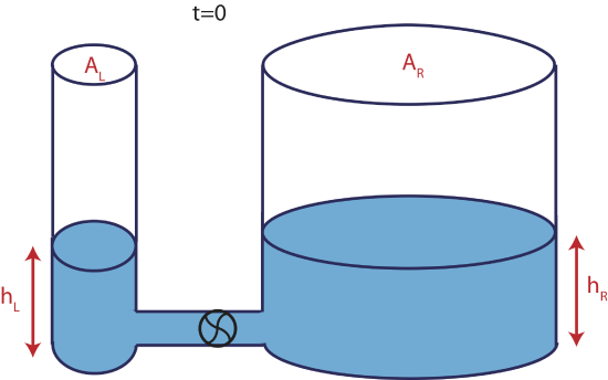
Two cylinders below have different cross sectional areas, such that the area of cylinder on the right is nine times greater than the area of the cylinder on the left.  Initially the water levels are at 2m in both cylinders and the pump is turned off, such that \(h_L=h_R=2m\) at \(t=0\) in the figure below. The pump in this system can support a maximum height difference of 10 meters. When the pump is turned on, it pumps water from the right to the left cylinder. The main source of resistance is in the thin connecting pipe, which has a resistance of \(1.6\times 10^4\dfrac{Js}{m^6}\).  The density of water is \(1000\dfrac{kg}{m^3}\).

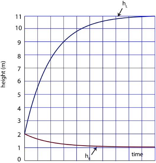
a) Make a plot of the water levels, \(h_R\) and \(h_L\), as a function of time from the moment the pump is turned on until the system reaches equilibrium. Make sure to mark numerical values for initial and final heights. (You do not need to derive any equations here.)

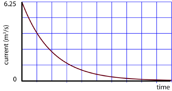
b) Likewise, make a plot of current as a function of time. Make sure to mark numerical values for initial and final currents.  

c) What will be the height in the left and the right cylinders after 2 half-lives?

Solution

The flow rate \(I\) is related to rate of change of height since, \(I=\dfrac{dV}{dt}=A\dfrac{dh}{dt}\) since \(V=Ah\). In this system the rate of change of the height is proportional to the height, the change is exponential, and approaching a total height difference of 10m as stated in the problem. The magnitude of the current flowing out of the right standpipe is equal to the current flowing into the left standpipe, except the volume is increasing in the left cylinder and decreasing in the right one.  This is accounted by the minus sign shown here:

\(I=\dfrac{dV_L}{dt}=-\dfrac{dV_R}{dt}\)

\(I=A_L\dfrac{dh_L}{dt}=-A_R\dfrac{dh_R}{dt}\)

Plugging in \(A_R=9A_L\):

\(\dfrac{dh_L}{dt}=-9\dfrac{dh_R}{dt}\)

We can rewrite the above equation in terms of change in height, starting at initial height and going to a maximum value:

\(h_{L,max}-h_0=-9(h_{R,min}-h_0)\)

Thus, the height in the left cylinder will increase nine times more than the height in the right one will decrease. Also, once the system reaches equilibrium:

\(h_{L,max}-h_{R,min}=10m\)

Using the two previous results and setting \(h_0=2m\) we get:

\((10+h_{R,min})-2=9(2-h_{R,min})\)

\(h_{R,min}+8=18-9h_{R,min}\)

\(h_{R,min}=1m\)

and

\(h_{L,max}=h_{R,min}+10m=11m\)

The plot for \(h_L\) and \(h_R\) is shown below.

b) When the pump is first turned on, this sets the initial current. Initially, there is no change in head across the system since the water levels are the same in both cylinders. Applying the Bernoulli equation across the thin pipe we get:

\(0=\tilde{E}_{\text{pump}} – I_0R\) 

so

\(I_0=\dfrac{\tilde{E}_{\text{pump}}}{R}\) 

We can also solve for \(\tilde{E}_{\text{pump}}\), since when the system reaches its equilibrium state the current goes to zero, and the height difference between the two pipes approaches 10m. Applying Bernoulli equation at equilibrium we get:

\(\tilde{E}_{\text{pump}}=\rho g(h_L-h_R)=1000\dfrac{kg}{m^3}\times 10\dfrac{m}{s^3}\times 10m=1.0\times 10^5 \dfrac{J}{m^3}\)

Solving for initial current we find:

\(I_0=\dfrac{\tilde{E}_{\text{pump}}}{R}=\dfrac{1.0\times 10^5 \dfrac{J}{m^3}}{1.6\times 10^4\dfrac{Js}{m^6}}=6.25\dfrac{m^3}{s}\) 

Thus the current starts at its initial values of \(6.25\dfrac{m^3}{s}\) and approaches zero exponentially as shown below.

c) After one half-life the heights will be halfway between its initial and final values. The left cylinder starts at 2m and ends at 11m. The height at one half-life is:

 \(h_L(t=t_{1/2})=h_0+\dfrac{h_{max}-h_0}{2}=2+\dfrac{11-2}{2}=6.5m\). 

For the right cylinder which starts at 2m and ends at 1m, after one half-life it will be at 2-1/2=1.5m. 

\(h_R(t=t_{1/2})=h_0-\dfrac{h_0-h_{min}}{2}=2-\dfrac{2-1}{2}=1.5m\). 

After another half-life the height for the left cylinder has to be halfway between 6.5m and 11m:

 \(h_L(t=2t_{1/2})=6.5+\dfrac{11-6.5}{2}=8.75m\). 

For the right cylinder the height is halfway between 1.5m and 1m which is:

\(h_R(t=2t_{1/2})=1.5-\dfrac{1.5-1}{2}=1.25m\). 

We saw two specific examples above of fluid flow exhibiting exponential change behavior. In one situation a pump was used to store water in one cylinder and in another the stored water flowed from one cylinder to another.  We will now introduced analogous situations for electric change flow and make connections to these two fluid examples.