5.10: Exponential Charge Flow

Charging Capacitor

When we discussed electric circuits earlier in this chapter we limited ourselves to circuits with batteries, wires, and resistors resulting in steady-state charge flow. We will now consider another circuit component, the capacitor. Capacitors are useful because they can store electric energy and release that stored energy quickly. Batteries store energy too, they just let it trickle out over a relatively long time. When you take a photograph with a flash, you may have noticed a high-pitched whine as the camera charged a capacitor. The capacitor then discharges a large burst of energy to light the flashbulb. Capacitors store energy by accumulating charge on two conducting plates, a net positive charge on one plate and a net negative charge on the other. Like charges repel each other, so it makes sense that as the charge builds up on each plate, it becomes increasingly difficult to add more charge. Or if you think about a capacitor that is already charged, at first there will be a large accumulation of charge pushing charges off the plates, and as the charges move the “pressure” pushing them will decrease. Here is another situation where the change in an amount is related to the amount already present. 

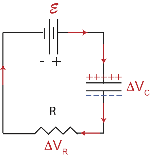
Figure 5.10.1 shows a typical RC circuit where a battery, a capacitor, and a resistor are all connected in series. The two parallel lines used to symbolize a capacitor represent the two conducting parallel plates with the space in between filled with an insulator. Charge cannot move across the capacitor since the insulating material does not allow charge to move across it. When the circuit is initially connected, electrons from the plate closest to the positive terminal of the battery get pulled to the positive terminal. This leaves behind a depletion of electrons on that plate making the net charge positive, as shown below. The red arrows represent the direction of current, which is the motion of positive charge carriers in the opposite direction of the motion of electrons. An analogous situation is occurring with the other other plate where electrons move from the negative terminal of the battery to the plate causing an accumulation of negative charge there. Thus, current flows toward the negative terminal at the same rate as it flows away from the positive terminal of the battery, charging the capacitor. We can consider this a closed circuit the same way we did for circuits without a capacitor. Although, charge is not moving across the capacitor, there is a uniform direction of charge flow in this circuit. Current does not technically flow through the battery either, there is a chemical reaction that occurs in the battery which keeps it at a fixed emf.

Figure 5.10.1: Charging Capacitor.

Let us think move deeply about the behavior of current as a function of time. Initially, the capacitor is not charged, and the two plates easily become charged. However, as the charges build up on each plate, the like charges repel each other on each plate, and it becomes harder to add more charge. So the current per unit time decreases until the force that pushing the charges onto the plate balances the force repelling those charges, resulting in zero net charge movement or current. Analogously, think back to the scenario in Figure 5.9.4. As the pump pushed water to the right cylinder, gravity was pulling the fluid back down, which made it harder for the pump to push more water upward, until the two effects were balanced. This is analogous to this RC circuit scenario, as the battery pushes charge onto the capacitor, the accumulated charge pushes those charges back, until the two effects become balanced, the emf of the battery will be equal to the voltage across the capacitor.

You can also think about this RC circuit in terms of the loop rule which still applies there:

\[\mathcal E +\Delta V_C+\Delta V_R=0\label{RC-charge}\]

Initially the capacitor is not charged, \(\Delta V_C=0\), so all the voltage drops across the resistor, \(\Delta V_R=-I_0R=-\mathcal E\), exactly how a simple circuit without a capacitor would behave. The initial current is then \(I_0=\dfrac{\mathcal E}{R}\). At equilibrium the voltage across the capacitor will equal to the emf of the battery, \(\mathcal E=-\Delta V_C\). Since no voltage will drop across the resistor, the current will go to zero.

How much charge exactly can accumulate on a capacitor? Not all capacitors are made equally, some are able to hold more charge than others. The property that determines how much charge a capacitor can hold when charged with some battery is known as capacitance, \(C\), which is given by:

\[C=\dfrac{Q}{\Delta V}\label{C}\]

The unit of capacitance is called a farad, which is abbreviated as "F", where \(F=\dfrac{C}{V}\). A capacitor with a large capacitance is able to store more charge per voltage difference. Capacitance is proportional to the area of the capacitor plate, the larger the area the more charges can spread out without repelling each other. This is analogous to the area of the cylinder, the larger the area the more volume can be stored in the cylinder. In addition, capacitance is inversely proportional to the distance between the two plates. As the plates are moved closer together, there is an additional attractive force between the two plates since they have opposite charge. This attraction allows more charge to be added.

Using the known expressions for the voltage drops across the capacitor and resistor and rewriting Equation \ref{RC-charge}, we get:

\[\mathcal E-\dfrac{Q}{C}-IR=0\]

Expressing current as the rate of change of charge, \(I=\dfrac{dQ}{dt}\) and solving for \(I\) we arrive at:

\[I(t)=\dfrac{dQ}{dt}=\dfrac{\mathcal E}{R}-\dfrac{Q}{RC}\label{It-RC-charge}\]

We once again have an expression that shows the dependence the rate of charge of some amount, here the rate of charge, \(\dfrac{dQ}{dt}\) on the amount of charge, \(Q\). The equation above has a similar form to Equation 5.9.15 for the rate of volume change in the two cylinder system. Applying a similar procedure to solve the differential Equation \ref{It-RC-charge} as we did for the cylinder system, we arrive at the following expression for charge as a function of time:

\[Q(t) = \mathcal E C\Big[1-\exp{\Big(-\dfrac{t}{RC}\Big)}\Big]\label{Qt}\]

Using the definition of current and taking the derivative of Equation \ref{Qt} we find that current has the following expression as a function of time:

\[I(t)=\dfrac{\mathcal E}{R}\exp{\Big(-\dfrac{t}{RC}\Big)}\label{Icharge}\]

The time constant is given by \(\tau=RC\) resulting in a half-life for the RC circuit:

\[t_{1/2}=RC\ln 2\]

Note the similarity between the way current behaves when a pump is used to store water in a cylinder (Equation 5.9.18) and when a battery is used to charge a capacitor (Equation \ref{Icharge}). In both cases the current starts with an initial maximum value which is proportional to the strength of the pump or battery and inversely proportional to the amount of resistance present that impedes the flow. Also, in both situations the rate of charge of current is proportional to the amount of current is present at a given time, which leads to exponential decay of the current to zero. An equilibrium state of zero current is reached when the strength of the pump or battery is balanced by an opposing force, gravity in the case of the fluid system and electric force in the case of an RC circuit. Both situations have a half-life which is determined by the properties of the system. A longer half-life for the water storing system is determined by a larger area allowing for a greater volume to be stored which takes more time and larger resistance making the flow slower. For the RC circuit the half-life is increased by a larger capacitance allowing more storage of charge which take more time, and resistance which slows down the current causing slower decay. It is fascinating that these two seeming different situations have extremely similar physical behavior.

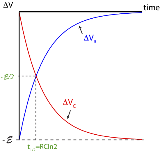
Conceptually, we can argue that the voltage across the capacitor starts and zero and approaches \(-\mathcal E\) exponentially while the voltage across the resistor starts at \(-\mathcal E\) and approaches zero exponentially as shown below in Figure 5.10.2.  Mathematically, we can use the above results to get an expression for voltage as a function of time.  Using Equations \ref{C} and \ref{Qt} we can find the voltage across the capacitor as a function of time:

\[\Delta V_C(t)=-\dfrac{Q(t)}{C}=-\mathcal E\Big[1-\exp{\Big(-\dfrac{t}{RC}\Big)}\Big]\]

And using, \(\Delta V_R=-IR\) and Equation \ref{Icharge} we find the following expression of the voltage drop across the resistor as a function of time:

\[\Delta V_R(t)=-\mathcal E\exp{\Big(-\dfrac{t}{RC}\Big)}\]

When we add the two equations above we find that they add up to \(-\mathcal E\). This is because energy is conserved during the entire process and the loop rule given in Equation \ref{RC-charge} applies at all times.  You can see this in Figure 5.10.2 below. In the figure the half-life is also labeled at the time when the voltage for both the resistor and capacitor reaches \(-\mathcal E/2\).

Figure 5.10.2: Voltages when Capacitor is Charging.

Discharging Capacitor

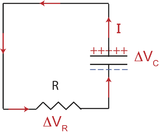
Now suppose we take the capacitor that was charged in a circuit in Figure 5.10.1, disconnected from a battery, and connected to just to a resistor as shown in Figure 5.10.3 below. In this case electrons from the negatively charged plate will be attracted to the positive plate and flow accordingly. Since current is the opposite direction of electrons, current will flow in the counterclockwise direction in the circuit below. The system will come to equilibrium when there is no longer a net charge on the two plates, resulting in no flow of electric charge, discharging the capacitor. Remember, a current flows when there is a attractive electric force present, such as a terminal of a battery or a charged plate in this case of a discharging capacitor.

Figure 5.10.3: Discharging Capacitor.

For this circuit the loop rule is:

\[\Delta V_C+\Delta V_R=0\label{RC-discharge}\]

Since the voltage across a resistor in the direction of current is always negative, the voltage across the capacitor has to be positive. If you follow the direction of the current in Figure 5.10.3 it goes from the negative plate to the positive plate, the same way the current in Figure 5.10.1 flows from the negative to the positive terminal of a battery resulting in a positive emf with the loop rule is applied.  In Figure 5.10.1 the current "flows" from the positive to the negative plate of the capacitor resulting in a negative change in the voltage of the capacitor in that case.

Alert

The voltage across a capacitor is always negative when it is charging and is positive when it is discharging when following the direction of current.

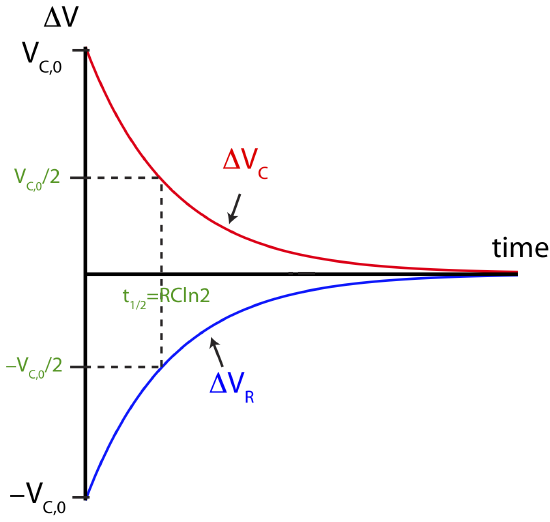
The voltage across the capacitor for the circuit in  Figure 5.10.3 starts at some initial value, \(V_{C,0}\), decreases exponential with a time constant of \(\tau=RC\), and reaches zero when the capacitor is fully discharged. For the resistor, the voltage is initially \(-V_{C,0}\) and approaches zero as the capacitor discharges, always following the loop rule so the two voltages add up to zero. This behavior is depicted in Figure 5.10.4 below. The half-life is also indicated when the voltages reach half of their initial value for both the resistor and the capacitor. 

Figure 5.10.4: Voltages when Capacitor is Discharging.

If you are more keen on showing it mathematically, start with Equation \ref{RC-discharge}, and follow the method outlined in the derivations shown in this section, to obtain mathematical exponential decay equations for charge across the capacitor, voltages across the capacitor and resistance, and the current. In this case a capacitor discharging is analogous to a cylinder with stored water flowing out to reach equilibrium as described in Figure 5.9.2.

Example \(\PageIndex{3}\)

Shown here is a circuit that contains a \(5V\) battery, a \(2F\) capacitor, several resistors with the same resistance \(R\), and two switches. Assume the capacitor is initially discharged.

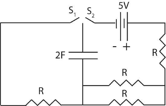
a) Initially the switch, S2, is closed while S1 remains open.  It takes 9 seconds for the capacitor to charge to 2 volts in this case. Once the capacitor is fully charged, S2 is open and S1 is closed. How long will it take the capacitor to reach 2.5 volts after S1 is closed?

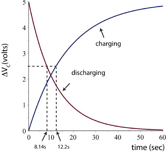
b) On the same plot, make a graph of the magnitude of the voltage across the capacitor as it charges and as it discharges in this circuit. Assume both processes start at t=0.  Mark at least one half-life with a numerical value.

Solution

 

a) To solve this problem, we first need to use the information given about the charging RC circuit to find the resistance R, since we have some information about the time it takes to discharge. Once we know R, we can find the half-life of the discharging circuit. 

The magnitude of voltage across a capacitor as it charges is:

\(|\Delta V_C|=\mathcal E \Big[1-\exp{\Big(-\dfrac{t}{R_{eq}C}\Big)}\Big]\)

We are given that at t=9sec, \(|\Delta V_C(9 s)|=2V\). Also, the equivalent resistance for the circuit when only S2 is closed is \(R_{eq}=R+\dfrac{R}{2}=\dfrac{3}{2}R\). Plugging these values into the equation above we get:

\(2V=5V\Big[1-\exp{\Big(-\dfrac{9 s}{3R/2\times 2F}\Big)}\Big]=5V\Big[1-\exp{\Big(-\dfrac{3}{R}\dfrac{s}{F}\Big)}\Big]\)

Solving for R:

\(\exp{\Big(-\dfrac{3}{R}\dfrac{s}{F}\Big)}=1-\dfrac{2}{5}=\dfrac{3}{5}\)

\(-\dfrac{3}{R}\dfrac{s}{F}=\ln\Big(\dfrac{3}{5}\Big)=-0.51\)

\(R=5.87\Omega\)

For the discharging circuit, there is only one resistor, so:

\(t_{1/2}=\ln 2 RC=\ln 2\times 5.87\Omega\times 2F=8.14 s\)

Thus, it will take 8.14 seconds for the capacitor to discharge to half of time maximum voltage of 5V, which is 2.5V.

b) For the charging circuit the half life is:

\(t_{1/2}=\ln 2 R_{eq}C=\ln 2\dfrac{3}{2}RC=\ln 2\times 5.87\dfrac{3}{2}\Omega\times 2F=12.2 s\)

The plots with the half-lives marked are shown below.

Other Systems

In each of these phenomena  we can understand the change by applying the basic ideas of the exponential change model. The fact that each version of the equation looks a bit different can easily hide that fact that the ideas underlying how the system changes are the same. The advantage of understanding the underlying behavior makes it possible for you to recognize the general pattern, even though the symbols are different or the equation is written differently.

Another example that displays exponential change is the the cooling of objects. Most of us have observed that an unfinished cup of hot coffee or tea will cool down to room temperature eventually. What might not be so obvious without taking some data is that the rate of cooling depends on the temperature difference between the hot object and its environment. So the hotter the cup of coffee, and the colder the room, the faster heat will move from the coffee to the room. This is known as Newton’s Law of Cooling given by:

\[\Delta T(t) = \Delta T_0 e^{-t/\tau}\]

where \(\Delta T\) is the temperature difference between the object and its environment. So as the hot object approaches the temperature of its environment, the rate of cooling decreases and asymptotically approaches zero. The temperature difference behaves exactly like the example of nuclear decay, fluid flow examples described in this section, and RC circuits.