2.3: Computing Potential Fields for Known Charge Distributions

Electrostatic Potential Field of Straight Line Segment of Uniform Density

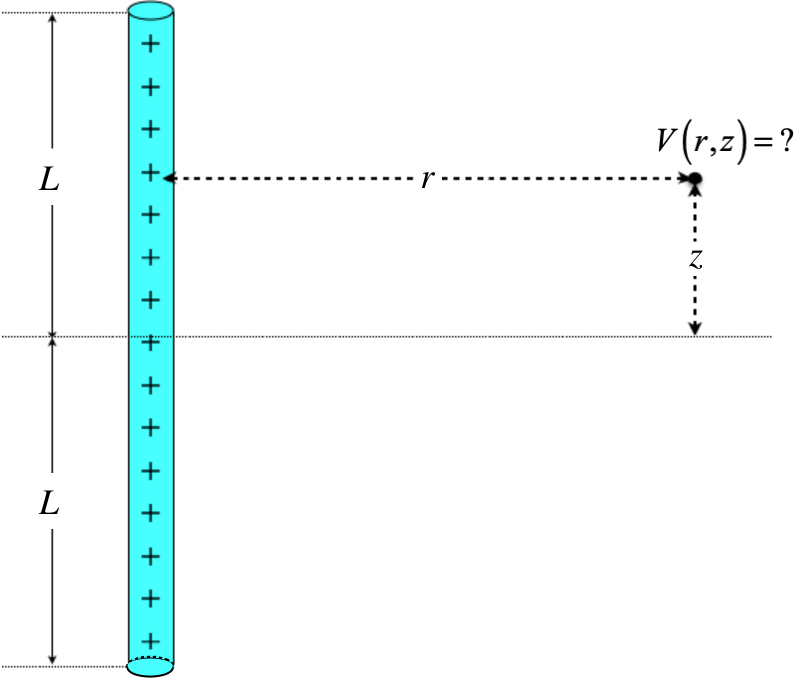
We return to the problem we first solved way back in Section 1.3. Actually, we are going to take it a step further than we did before, which will show the power of approaching the problem of computing fields with potentials. In our direct calculation of the electric field, we punted the computation of the \(z\)-component due to the lack of symmetry. It's not that it was impossible to do, but the vector element of the calculation was daunting, and in any case we now have a different approach that is easier to use. So the physical set-up is the same as before – a uniform linear segment of charge located along the \(z\)-axis from \(z=-L\) to \(z=+L\). But now we seek the potential field at a position a distance \(r\) from the \(z\)-axis, and a distance \(z\) from the \(\left(x,y\right)\) plane. We still have cylindrical symmetry, which means we don't have to specify the polar angle of the position of the point in space.

Figure 2.3.1a – Electrostatic Potential Field of a Uniform Line Segment

We start the same way as we did for the electric field – identifying an element of charge, setting up a coordinate system, and determining the distance from the point charge to the point in space:

Figure 2.3.1b – Electrostatic Potential Field of a Uniform Line Segment

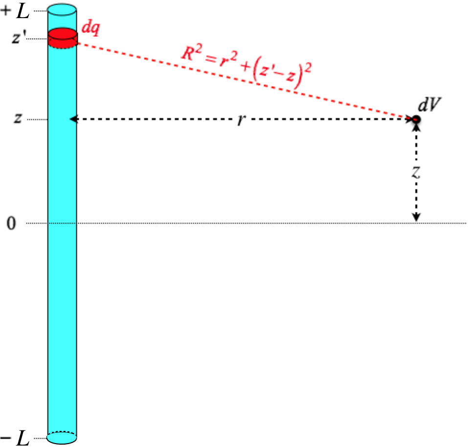
To start the math, we make several notes: First, unlike the electric field, we are not dealing with vectors, so we don't have to track components (yay!). Second, we need to reference the zero point of potential, and we will do so with the usual \(V\left(\infty\right)=0\). Finally, it should be noted that it is a bit awkward to integrate over the \(z\) variable, while our final answer is a function of the \(z\) component of the position in space, so we have named our integration variable \(z'\).

\[\left. \begin{array}{l} dq=\lambda \;dz' \\dV=\dfrac{dq}{4\pi \epsilon_o R} \end{array} \right\} \;\;\; \Rightarrow \;\;\; V\left(r,z\right) = \int\limits_{-L}^{+L} \dfrac{\lambda\;dz'}{4\pi \epsilon_o \sqrt{r^2+\left(z'-z\right)^2}} \]

With a substitution of \(u\equiv z'-z\), the integral becomes easy to look up in an integral table:

\[V\left(r,z\right) = \dfrac{\lambda}{4\pi \epsilon_o} \int\limits_{-z-L}^{-z+L} \dfrac{du}{\sqrt{r^2+u^2}} = \dfrac{\lambda}{4\pi \epsilon_o}\left[\ln\left(\sqrt{r^2+u^2}+u\right)\right]_{-z-L}^{-z+L} = \dfrac{\lambda}{4\pi \epsilon_o} \ln\left(\dfrac{\sqrt{r^2+\left(z-L\right)^2}+L-z}{\sqrt{r^2+\left(z+L\right)^2}-L-z}\right)\]

Okay, so that's quite a mess, but consider this: The set-up and the math to get here was not all that tough, and we have so much more information here. This is the potential field throughout all of space. When we calculated the electric field for this charge distribution, we were somewhat daunted by the lack of symmetry that occurs off the \(x\)-axis, making dealing with the vector components off the \(x\)-axis problematic (not impossible, but certainly not much fun). And now if we want the electric field at any point in space (the \(\widehat z\) component as well as the \(\widehat r\) component!), we only need to take derivatives, since the potential field is related to the electric field through the gradient.

Example \(\PageIndex{1}\)

If we take the solution found in Example 1.3.2 and make the cylinder infinitesimally thin (\(a\rightarrow 0\)), we get that the electric field magnitude on the \(z\)-axis for a uniformly charged rod of length \(2L\) is:

\[E = \dfrac{Q}{8\pi\epsilon_oL}\left[\dfrac{1}{z-L} - \dfrac{1}{z+L}\right]\nonumber\]

1. Find the electrostatic potential on the \(z\)-axis for this collection of charge.
2. Use the electrostatic potential on the \(z\)-axis to show that the electric field there comes out to what we found previously.

Solution

a. We can start from scratch an perform the integral, but why do this, when we have a general solution for this charge distribution above? All we need to do is take the limit of \(r\rightarrow 0\) and we will be confined to the \(z\)-axis:

\[\lim\limits_{r\rightarrow 0}\; V\left(r, z\right) = \dfrac{\lambda}{4\pi \epsilon_o} \lim\limits_{r\rightarrow 0}\; \ln\left(\dfrac{\sqrt{r^2+\left(z-L\right)^2}+L-z}{\sqrt{r^2+\left(z+L\right)^2}-L-z}\right) = \dfrac{\lambda}{4\pi \epsilon_o} \ln\left(\dfrac{\sqrt{0+\left(z-L\right)^2}+L-z}{\sqrt{0+\left(z+L\right)^2}-L-z}\right) = \dfrac{\lambda}{4\pi \epsilon_o} \ln\left(\dfrac{0}{0}\right) \nonumber\]

We have an indeterminate form, so we need to employ l'Hôpital's rule:

\[\lim\limits_{r\rightarrow 0}\; \ln\left[\dfrac{f\left(r\right)}{g\left(r\right)}\right] = \ln\left[\lim\limits_{r\rightarrow 0}\dfrac{f\left(r\right)}{g\left(r\right)}\right] = \ln\left[\lim\limits_{r\rightarrow 0}\dfrac{f'\left(r\right)}{g'\left(r\right)}\right] = \ln\left[\lim\limits_{r\rightarrow 0}\dfrac{\dfrac{r}{\sqrt{r^2+\left(z-L\right)^2}}+0}{\dfrac{r}{\sqrt{r^2+\left(z+L\right)^2}}+0}\right] = \ln\left[\lim\limits_{r\rightarrow 0}\dfrac{\sqrt{r^2+\left(z+L\right)^2}}{\sqrt{r^2+\left(z-L\right)^2}}\right] = \ln\left[\dfrac{z+L}{z-L}\right]\nonumber\]

\[\Rightarrow \;\;\; \lim\limits_{r\rightarrow 0}\; V\left(r, z\right) = \dfrac{\lambda}{4\pi \epsilon_o}\left[\ln\left(z+L\right) - \ln\left(z-L\right)\right]\nonumber\]

b. To find the component of the electric field along the \(z\)-axis (which we can tell from symmetry is the only component of the field on that axis), we take the negative derivative with respect to \(z\):

\[E_z = -\dfrac{\partial V}{\partial z} = \dfrac{\lambda}{4\pi \epsilon_o}\left[\dfrac{1}{z-L} - \dfrac{1}{z+L}\right]\nonumber\]

Plugging-in \(\lambda = \frac{Q}{2L}\) for the uniform charge density gives us the electric field shown above.

[It should be noted that it is a better idea to perform the gradient operation before taking a limit (in this case \(r\rightarrow 0\)), because some information about the potential that is used in the electric field can be lost when the limit is taken first. In this particular case, symmetry ensured that the electric field would only point along the \(z\)-direction on the \(z\)-axis, so it was safe (and mathematically more expedient) to take the limit first.]

Electrostatic Potential Field of Long Straight Line of Uniform Density

As with the case of the electric field, the potential for a long ("infinite") line of charge is of importance to us. So the natural step to take is to simply use the result above, and take the limit as \(L\rightarrow \infty\). But when we try to do this, we find that the limit diverges. This is puzzling, as the electric field comes out right from the gradient, and it doesn't diverge in the limit. The answer has to do with our choice of where the potential is chosen to be zero, and we can fix the problem by simply choosing another position for the zero potential. Let's choose the position for zero potential to be: \(r=r_o,\;z=0\). If we do this, we get a revised version of our potential function for the line segment:

\[V\left(r,z\right) = \dfrac{\lambda}{4\pi \epsilon_o} \left[\ln\left(\dfrac{\sqrt{r^2+\left(z-L\right)^2}+L-z}{\sqrt{r^2+\left(z+L\right)^2}-L-z}\right)-\ln\left(\dfrac{\sqrt{r_o^2+L^2}+L}{\sqrt{r_o^2+L^2}-L}\right)\right]\]

The reader can easily confirm that in fact \(V\left(r_o,0\right)=0\). It's not immediately clear how this rescues our limit of \(L\rightarrow\infty\). To see how this happens requires a bit of math, but it is useful to see, so here goes... First, it's clear that when the line becomes infinitely-long, the value of \(z\) is irrelevant, and might as well be set to zero. Plugging this in, and dividing the numerator and denominator of both natural log arguments by \(L\) simplifies our potential to:

\[V\left(r\right) = \dfrac{\lambda}{4\pi \epsilon_o} \left[\ln\left(\dfrac{\sqrt{1+\frac{r^2}{L^2}}+1}{\sqrt{1+\frac{r^2}{L^2}}-1}\right)-\ln\left(\dfrac{\sqrt{1+\frac{r_o^2}{L^2}}+1}{\sqrt{1+\frac{r_o^2}{L^2}}-1}\right)\right]\]

Now we make use of the following expansion to first order for very small \(\epsilon\):

\[\sqrt{1+\epsilon}\approx 1+\frac{1}{2}\epsilon \]

In our case, of course the ratios with \(L^2\) in the denominator are very small, so we get:

\[V\left(r\right) = \dfrac{\lambda}{4\pi \epsilon_o} \left[\ln\left(\dfrac{1+\frac{r^2}{2L^2}+1}{1+\frac{r^2}{2L^2}-1}\right)-\ln\left(\dfrac{1+\frac{r_o^2}{2L^2}+1}{1+\frac{r_o^2}{2L^2}-1}\right)\right] = \dfrac{\lambda}{4\pi \epsilon_o} \left[\ln\left(4\dfrac{L^2}{r^2}+1\right)-\ln\left(4\dfrac{L^2}{r_o^2}+1\right)\right] = \dfrac{\lambda}{4\pi \epsilon_o}\ln\left(\dfrac{\frac{1}{r^2}+\frac{1}{4L^2}}{\frac{1}{r_o^2}+\frac{1}{4L^2}}\right)\]

Now take our limit of \(L\rightarrow\infty\) at last, to obtain:

\[V\left(r\right) = \dfrac{\lambda}{4\pi \epsilon_o} \ln\left(\dfrac{r_o^2}{r^2}\right) = \dfrac{\lambda}{2\pi \epsilon_o} \ln\left(\dfrac{r_o}{r}\right)\]

We will find this result quite useful for cylindrical symmetries. It clearly still vanishes at \(r=r_o\) and its negative gradient gives the correct field for the long line of uniform charge (Equation 1.3.21).

As with the case of electric fields, we can also compute potential scalar fields for non-uniform charge distributions. The reader is encouraged to go back to re-work Example 1.3.4 (for which the density was non-uniform) by starting with computing the electrostatic potential field.