
2.4: Capacitance
- Page ID
- 17357

\( \newcommand{\vecs}[1]{\overset { \scriptstyle \rightharpoonup} {\mathbf{#1}} } \)
\( \newcommand{\vecd}[1]{\overset{-\!-\!\rightharpoonup}{\vphantom{a}\smash {#1}}} \)
\( \newcommand{\dsum}{\displaystyle\sum\limits} \)
\( \newcommand{\dint}{\displaystyle\int\limits} \)
\( \newcommand{\dlim}{\displaystyle\lim\limits} \)
\( \newcommand{\id}{\mathrm{id}}\) \( \newcommand{\Span}{\mathrm{span}}\)
( \newcommand{\kernel}{\mathrm{null}\,}\) \( \newcommand{\range}{\mathrm{range}\,}\)
\( \newcommand{\RealPart}{\mathrm{Re}}\) \( \newcommand{\ImaginaryPart}{\mathrm{Im}}\)
\( \newcommand{\Argument}{\mathrm{Arg}}\) \( \newcommand{\norm}[1]{\| #1 \|}\)
\( \newcommand{\inner}[2]{\langle #1, #2 \rangle}\)
\( \newcommand{\Span}{\mathrm{span}}\)
\( \newcommand{\id}{\mathrm{id}}\)
\( \newcommand{\Span}{\mathrm{span}}\)
\( \newcommand{\kernel}{\mathrm{null}\,}\)
\( \newcommand{\range}{\mathrm{range}\,}\)
\( \newcommand{\RealPart}{\mathrm{Re}}\)
\( \newcommand{\ImaginaryPart}{\mathrm{Im}}\)
\( \newcommand{\Argument}{\mathrm{Arg}}\)
\( \newcommand{\norm}[1]{\| #1 \|}\)
\( \newcommand{\inner}[2]{\langle #1, #2 \rangle}\)
\( \newcommand{\Span}{\mathrm{span}}\) \( \newcommand{\AA}{\unicode[.8,0]{x212B}}\)
\( \newcommand{\vectorA}[1]{\vec{#1}} % arrow\)
\( \newcommand{\vectorAt}[1]{\vec{\text{#1}}} % arrow\)
\( \newcommand{\vectorB}[1]{\overset { \scriptstyle \rightharpoonup} {\mathbf{#1}} } \)
\( \newcommand{\vectorC}[1]{\textbf{#1}} \)
\( \newcommand{\vectorD}[1]{\overrightarrow{#1}} \)
\( \newcommand{\vectorDt}[1]{\overrightarrow{\text{#1}}} \)
\( \newcommand{\vectE}[1]{\overset{-\!-\!\rightharpoonup}{\vphantom{a}\smash{\mathbf {#1}}}} \)
\( \newcommand{\vecs}[1]{\overset { \scriptstyle \rightharpoonup} {\mathbf{#1}} } \)
\(\newcommand{\longvect}{\overrightarrow}\)
\( \newcommand{\vecd}[1]{\overset{-\!-\!\rightharpoonup}{\vphantom{a}\smash {#1}}} \)
\(\newcommand{\avec}{\mathbf a}\) \(\newcommand{\bvec}{\mathbf b}\) \(\newcommand{\cvec}{\mathbf c}\) \(\newcommand{\dvec}{\mathbf d}\) \(\newcommand{\dtil}{\widetilde{\mathbf d}}\) \(\newcommand{\evec}{\mathbf e}\) \(\newcommand{\fvec}{\mathbf f}\) \(\newcommand{\nvec}{\mathbf n}\) \(\newcommand{\pvec}{\mathbf p}\) \(\newcommand{\qvec}{\mathbf q}\) \(\newcommand{\svec}{\mathbf s}\) \(\newcommand{\tvec}{\mathbf t}\) \(\newcommand{\uvec}{\mathbf u}\) \(\newcommand{\vvec}{\mathbf v}\) \(\newcommand{\wvec}{\mathbf w}\) \(\newcommand{\xvec}{\mathbf x}\) \(\newcommand{\yvec}{\mathbf y}\) \(\newcommand{\zvec}{\mathbf z}\) \(\newcommand{\rvec}{\mathbf r}\) \(\newcommand{\mvec}{\mathbf m}\) \(\newcommand{\zerovec}{\mathbf 0}\) \(\newcommand{\onevec}{\mathbf 1}\) \(\newcommand{\real}{\mathbb R}\) \(\newcommand{\twovec}[2]{\left[\begin{array}{r}#1 \\ #2 \end{array}\right]}\) \(\newcommand{\ctwovec}[2]{\left[\begin{array}{c}#1 \\ #2 \end{array}\right]}\) \(\newcommand{\threevec}[3]{\left[\begin{array}{r}#1 \\ #2 \\ #3 \end{array}\right]}\) \(\newcommand{\cthreevec}[3]{\left[\begin{array}{c}#1 \\ #2 \\ #3 \end{array}\right]}\) \(\newcommand{\fourvec}[4]{\left[\begin{array}{r}#1 \\ #2 \\ #3 \\ #4 \end{array}\right]}\) \(\newcommand{\cfourvec}[4]{\left[\begin{array}{c}#1 \\ #2 \\ #3 \\ #4 \end{array}\right]}\) \(\newcommand{\fivevec}[5]{\left[\begin{array}{r}#1 \\ #2 \\ #3 \\ #4 \\ #5 \\ \end{array}\right]}\) \(\newcommand{\cfivevec}[5]{\left[\begin{array}{c}#1 \\ #2 \\ #3 \\ #4 \\ #5 \\ \end{array}\right]}\) \(\newcommand{\mattwo}[4]{\left[\begin{array}{rr}#1 \amp #2 \\ #3 \amp #4 \\ \end{array}\right]}\) \(\newcommand{\laspan}[1]{\text{Span}\{#1\}}\) \(\newcommand{\bcal}{\cal B}\) \(\newcommand{\ccal}{\cal C}\) \(\newcommand{\scal}{\cal S}\) \(\newcommand{\wcal}{\cal W}\) \(\newcommand{\ecal}{\cal E}\) \(\newcommand{\coords}[2]{\left\{#1\right\}_{#2}}\) \(\newcommand{\gray}[1]{\color{gray}{#1}}\) \(\newcommand{\lgray}[1]{\color{lightgray}{#1}}\) \(\newcommand{\rank}{\operatorname{rank}}\) \(\newcommand{\row}{\text{Row}}\) \(\newcommand{\col}{\text{Col}}\) \(\renewcommand{\row}{\text{Row}}\) \(\newcommand{\nul}{\text{Nul}}\) \(\newcommand{\var}{\text{Var}}\) \(\newcommand{\corr}{\text{corr}}\) \(\newcommand{\len}[1]{\left|#1\right|}\) \(\newcommand{\bbar}{\overline{\bvec}}\) \(\newcommand{\bhat}{\widehat{\bvec}}\) \(\newcommand{\bperp}{\bvec^\perp}\) \(\newcommand{\xhat}{\widehat{\xvec}}\) \(\newcommand{\vhat}{\widehat{\vvec}}\) \(\newcommand{\uhat}{\widehat{\uvec}}\) \(\newcommand{\what}{\widehat{\wvec}}\) \(\newcommand{\Sighat}{\widehat{\Sigma}}\) \(\newcommand{\lt}{<}\) \(\newcommand{\gt}{>}\) \(\newcommand{\amp}{&}\) \(\definecolor{fillinmathshade}{gray}{0.9}\)Definition of Capacitance
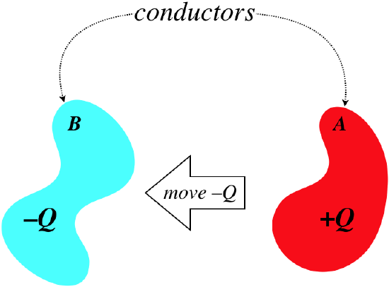
Imagine for a moment that we have two neutrally-charged but otherwise arbitrary conductors, separated in space. From one of these conductors we remove a handful of charge (say \(-Q\)), and place it on the other conductor.
Figure 2.4.1 – Charge Separated to Two Conductors
So now we have two conductors, one with a net charge of \(+Q\), and the other with a net charge of \(-Q\). Clearly there is an electric field pointing out of the former, and into the latter, with the field lines leaving and landing perpendicular to the surfaces.
Figure 2.4.2 – Field Between the Two Conductors
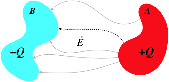
If we follow a field line leaving the positively-charged conductor and do a line integral along this field line until we reach the negatively-charged conductor, the result will be a decrease in electric potential, \(\Delta V\). That is, the positively-charged conductor will be an equipotential at a higher voltage than the equipotential that is the negatively-charged conductor.
\[V_A-V_B=\int\limits_A^B\overrightarrow E\cdot\overrightarrow{dl} \]
Now let's imagine what happens if we take an additional \(-Q\) from conductor \(A\) and move it over to conductor \(B\). What would we expect to see change in the electric field? We would expect the magnitude of the electric field to change, but the field lines should be shaped exactly the same. This is because the relative densities of charge at different locations on each conductor shouldn’t change, and the field lines still need to be perpendicular to the conducting surfaces.
Figure 2.4.3 – Doubling the Charge Separated Between the Conductors
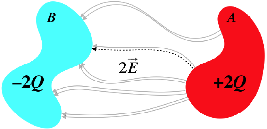
Consequently, when we compute the potential change using the same path as before (i.e. following the same field line) with twice the charge, the only thing that should be different is the magnitude of the electric field at each point, and this magnitude should be exactly twice as great (e.g. we know this is true at each conducting surface where the field strength is proportional to the charge density). We express this fact that the potential difference across two conductors is proportional to the charge they separate in a simple equation:
\[Q_{separated} \propto \Delta V \;\;\; \Rightarrow \;\;\; Q=C\Delta V\]
The constant \(C\) is called the capacitance of this two-conductor set-up. We associate this constant with the set-up because if the geometry is somehow changed (the conductors are pulled farther apart, one is rotated, the shape of one is altered, etc.), then the electric field lines from one to the other will change, and the line integral along one of those field lines will give a different potential difference, even though the same charge is separated. That is, the capacitance of a system of conductors is uniquely-defined by the physical structure of those conductors, but is unaffected by the amount of charge separated. The units of capacitance are obviously coulombs per volt, which is renamed for brevity to farads. A coulomb is a rather large amount of charge, and for most real-world applications of capacitance, we will see significantly less than a farad of capacitance, typically in the range of microfarads (\(\mu F\)).
Parallel-Plate Capacitor
While capacitance is defined between any two arbitrary conductors, we generally see specifically-constructed devices called capacitors, the utility of which will become clear soon. We know that the amount of capacitance possessed by a capacitor is determined by the geometry of the construction, so let’s see if we can determine the capacitance of a very simple capacitor – the parallel-plate capacitor.
Figure 2.4.4 – Parallel-Plate Capacitor
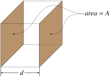
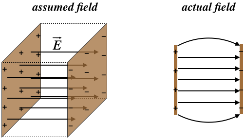
This kind of capacitor is modeled by two flat (obviously parallel) conducting plates, and while they are finite in extent, we approximate the fields between the plates with a uniform field. This approximation is quite good near the centers of the plates, but breaks down near the edges, where the field bows outward. This phenomenon (commonly referred to as fringe effects) plays a role that we will see later, but for now our approximation is that the field is uniform throughout the entire volume of the capacitor.
Figure 2.4.5 – Field Inside a Parallel-Plate Capacitor
While the capacitance depends only upon the structure of this capacitor, to figure out what the capacitance actually is, we need to place some charge on the plates, and compute the potential difference. We will then find that the ratio of these quantities is only a function of geometry. The field is uniform, which means that the field at the surface of one conductor is the same throughout the space between the conductors, and is the same at the other surface. But we already know what the field at the surface of a conductor is: \(E=\frac{\sigma}{\epsilon_o}\). If there is a total charge separation of \(Q\), then the uniform charge density is just that charge divided by the area of the conductor, giving:
\[ E=\dfrac{\sigma}{\epsilon_o} = \dfrac{Q}{A\epsilon_o} \]
From the electric field, we can compute the potential difference. Taking a straight-line path from the positive plate to the negative plate, the path integral is easy, as the electric field is constant, and the angle between the field and displacement is zero throughout the path:
\[voltage\;drop = \Delta V = V_A-V_B = \int\limits_A^B \overrightarrow E\cdot\overrightarrow{dl} = E\int\limits_A^B dl = E\;d\]
Plugging this in above gives:
\[ E = \dfrac{Q}{\epsilon_oA} = \dfrac{\Delta V}{d} \;\;\; \Rightarrow \;\;\; Q = \left(\dfrac{\epsilon_oA}{d}\right)\Delta V\]
The capacitance is the ratio of the charge separated to the voltage difference (i.e. the constant that multiplies \(\Delta V\) to get \(Q\)), so we have:
\[C_{parallel-plate} = \dfrac{\epsilon_oA}{d} \]
[Note: From this point forward, in the context of voltage drops across capacitors and other devices, we will drop the "\(\Delta\)" and simply use "\(V\)." That \(V\) represents a voltage difference and not an electrostatic potential at a point in space will be clear from context.]
Coaxial Cylindrical Capacitor
Looking at the final answer for the capacitance of the parallel-plate capacitor, we see that indeed it only depends upon the structure of the conducting surfaces – in particular, the cross-sectional area and their separation. To see that this particular formula for capacitance is unique to parallel-plate capacitors, it is helpful to look at another conductor structure. One that is common to find in practice is two coaxial conducting cylinders.
Figure 2.4.6 – Cylindrical Capacitor
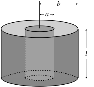
Once again we separated some charge across the conductors, and compute the potential drop between them. In this case, symmetry demands that the field is radial from the axis (it points outward if the inside conductor is the positively-charged one), although once again fringe effects occur near the edges, which we will ignore. We can use Gauss's law to show that the field is identical to that of a long line of charge with density \(\lambda\):
\[E\left(r\right)=\dfrac{\lambda}{2\pi\epsilon_o r}\]
The line density is the charge per unit length, so in terms of the separated charge and the dimensions of the cylinder, have simply \(\lambda \cdot l = Q\). As above, we can do a line integral from one plate to the other to get the voltage drop. Let's call the inner \(A\) and the outer cylinder \(B\) and assume the inner cylinder is positively-charged. Then we have:
\[V = \int\limits_A^B \overrightarrow E\cdot\overrightarrow{dl} = \int\limits_a^b E\left(r\right)dr = \dfrac{Q}{2\pi\epsilon_o l}\int\limits_a^b \dfrac{1}{r}dr = \dfrac{Q}{2\pi\epsilon_o l}\ln\left(\dfrac{b}{a}\right)\]
Notice that as soon as we realized that the field within this capacitor is the same as that of a long line of charge, we could have simply used our previous result, Equation 2.3.7. Simply plug in \(r=a\) for the potential of the smaller cylinder and \(r=b\) for the potential of the larger cylinder, and find the difference of the two.
The capacitance of this set-up is the ratio of the charge to the potential drop, so we have:
\[C=\dfrac{Q}{V} = \dfrac{2\pi\epsilon_o l}{\ln\left(\frac{b}{a}\right)}\]
This is quite different from case of a capacitor with a parallel-plate geometry.
Work Functions of Metals
At this point it seems appropriate to ask: “Why don’t the oppositely-charged plates draw charges off one another? That is, why don’t sparks fly across the capacitor gap?” It turns out that whenever we get into the nitty-gritty details of how charges behave on an atomic scale, things get complicated very fast. You will examine a bit of this when/if you move on to Physics 9D, but for now we'll say that the charges are held on the conductor by the nearby charges in the metal (it’s the protons holding the electrons to the metal). The grip these nearby charges have is not infinite, and the strength of their grip is measured by a quantity known as the work function of the metal. This measures the amount of energy that must be added to a single electron to get it to escape the surface of the metal.
As we build charge on the two plates (and hold the geometry fixed), the electric field grows, increasing the force on the charges. If enough charge is added to the plates, then this force is sufficient to overcome the work function, and electrons spark across the gap. It should be pointed out that this maximum capacity for charge is not what is being referred-to when using the word “capacitance,” though of course they are related – all else being equal, a capacitor with a higher capacitance will hold more charge before sparking. This sparking condition can also work another way: If the potential across the two plates is held fixed, and the gap is shortened, then since \(dV=-Edx\), the electric field gets stronger, and a spark can occur.
Energy Storage
What is the point of constructing capacitors? Energy storage. How do we know energy is stored in a capacitor? We take some charge away from one conductor and put it on the other, which means we are pulling charge away from opposite-sign charges, and pushing it toward same-sign charges. This requires putting in work, and accumulates electrical potential energy. We can calculate exactly how much energy is stored, and as always, we do so incrementally.
Figure 2.4.7 – Energy Accumulation in a Capacitor
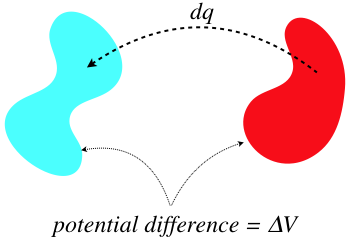
When we move an infinitesimal charge \(dq\) across a potential \(\Delta V\), the increase in energy is the product of these values. But the potential difference can also be written in terms of the charge on the conductors and the capacitance, the latter of which is a constant so long as the geometry of the conductors is unchanged.
\[dU = dqV = dq\left(\dfrac{q}{C}\right) \;\;\; \Rightarrow \;\;\; U = \int\limits_0^Q\dfrac{q\;dq}{C} = \dfrac{1}{2}\dfrac{Q^2}{C} \]
With the relation \(Q=CV\), we can rewrite this expression of potential energy two other ways. To summarize:
\[ U= \dfrac{1}{2}\dfrac{Q^2}{C} = \dfrac{1}{2}CV^2 = \dfrac{1}{2}QV \]
The most commonly-used of these expressions in practice is the second one, since we are typically handed a capacitor of a known capacitance, and want to know how much energy we can store in it when we apply a known voltage. Measuring the charge is not generally an easy thing to do (except indirectly, knowing C and V).
Example \(\PageIndex{1}\)
Imagine pulling apart two charged parallel plates of a capacitor until the separation is twice what it was initially. It should not be surprising that the energy stored in that capacitor will change due to this action. For the two cases given below, determine the change in potential energy. Also, provide a careful accounting of the energy: If the potential energy does down, explain where the energy goes, and if it goes up, explain where the energy comes from.
- the charged capacitor is not connected to anything that would allow it to change the charge on its plates
- the charged capacitor is connected to a device that adjusts the charge on the plates, such that the plates of the capacitor are held at a constant electric potential difference
- Solution
-
For both cases, increasing the separation changes the physical structure of the capacitor, and since the capacitance only depends upon the physical structure (not the charge or voltage), we use the parallel-plate equation:
\[C = \dfrac{\epsilon_o A}{d}\nonumber\]
Doubling the separation therefore reduces the capacitance to one-half its original value. We now use this fact for the two cases given.
a. Without the ability to adjust the amount of charge, it doesn't make sense to use \(U = \frac{1}{2}CV^2\) to compute the potential energy change, because both variables are changing at once. We therefore use:
\[\left. \begin{array}{l} U_{before} = \dfrac{1}{2}\dfrac{Q^2}{C} \\ U_{after} = \dfrac{1}{2}\dfrac{Q^2}{\frac{1}{2}C} \end{array} \right\}\;\;\; U_{after} =2U_{before} \nonumber\]
So the electric potential energy within the capacitor doubles, but where does this energy come from? Well, the plates are oppositely-charged, so they attract each other. Pulling them apart requires exertion – work must be done on the system. To compute the work done, we need to know the force required to barely get the plates to separate further (more force than this would accelerate the plates, which would bring unwanted kinetic energy into the calculation). This minimum force just equals the force of attraction between the plates, but what is this?
Consider a single charge \(q\) on one of the plates. It is in a uniform field caused by the other plate, so it feels a force toward the other plate equal to:
\[F_{single\;charge} = qE_{other\;plate} \nonumber\]
Of course, every charge on this same plate feels this force, so the total force on the plate is simply the sum of these forces:
\[F_{on\;plate\;A} = Q_{on\;plate\;A}E_{by\;plate\;B} \nonumber\]
But the field due to the other plate is not the same as the total field within the capacitor – the total field is a superposition of the fields due to both plates, and both plates contribute the same amount of field in the same direction, so in terms of the field in the capacitor, we have:
\[F_{on\;plate\;A} = Q_{on\;plate\;A}\left[\frac{1}{2}E_{total}\right] = \frac{1}{2}QE \nonumber\]
The charge doesn't change while the plates are pulled apart, so the electric field doesn't change either, which means that the force between the plates remains constant, making the work calculation easy. The amount of additional separation is \(d\), so:
\[W = \int \overrightarrow F\cdot \overrightarrow{dl} = F\Delta x \;\;\;\Rightarrow\;\;\; W=\left(\frac{1}{2}QE\right)\left(d\right) \nonumber\]
The quantity \(E\cdot d\) is the original potential difference \(V\). The energy put into the system by work is therefore \(\frac{1}{2}QV\), which equals precisely the potential energy the system started with, confirming that the potential energy is doubled.
b. Holding the potential between the plates fixed suggests using a different equation to determine the effect on the potential energy:
\[\left. \begin{array}{l} U_{before} = \dfrac{1}{2}CV^2 \\ U_{after} = \dfrac{1}{2}\left(\frac{1}{2}C\right)V^2 \end{array} \right\}\;\;\; U_{after} =\frac{1}{2}U_{before} \nonumber\]
This is a bit puzzling – clearly work must be done to separate the oppositely-charged plates, which adds energy to the system, but somehow the stored potential energy goes down?! The answer lies in the fact that to keep the potential the same as the plates separate, charge must leave the plates. Wherever this charge goes, its accumulation at that other place increases the potential energy there. So energy leaves the system and is stored as potential energy elsewhere.
To determine how much energy is gained by the "other place," we multiply the charge moved (which we know is half the charge on the capacitor, since its capacitance goes down by that factor and the voltage stays the same) by the potential difference:
\[\Delta U_{other\;place} = Q_{moved}V = +\frac{1}{2}QV \nonumber\]
This is the entirety of the energy that starts in the capacitor! But the energy doesn't end up with zero potential energy because there is work done in the separation. We can compute the work as we did in part (a), except that we need to keep in mind that the charge and electric field are changing as the plates are being separated. We know the relationship between the field and the charge, so with the voltage difference held constant, we have:
\[\left. \begin{array}{l} V = E\cdot x \\ E=\dfrac{\sigma}{\epsilon_o} = \dfrac{Q}{\epsilon_oA} \end{array} \right\}\;\;\; F= \frac{1}{2}QE = \frac{1}{2}\left(\epsilon_oAE\right)E = \dfrac{\epsilon_oAV^2}{2x^2}\nonumber\]
Now computing the work:
\[W = \int F\cdot dx = \int\limits_d^{2d} \left(\dfrac{\epsilon_oAV^2}{2x^2}\right)dx = \dfrac{\epsilon_oAV^2}{2}\int\limits_d^{2d} \dfrac{dx}{x^2} = +\dfrac{\epsilon_oAV^2}{4d}\nonumber\]
Plugging in \(C=\dfrac{\epsilon_oA}{d}\) shows that the work done is \(\frac{1}{2}\left(\frac{1}{2}CV^2\right)\), which is half the original stored energy. So in showing that an amount equal to the starting energy exits the capacitor with the charge, and half the original energy enters the system via work, we have confirmed that the final potential energy is half of what it was at the beginning.
Energy Density in Electric Fields
An alternative way to discuss energy storage is in terms of the electric field. The simplest way to see this is to look at the energy stored in a parallel-plate capacitor:
\[U=\frac{1}{2}CV^2=\frac{1}{2}\left(\dfrac{\epsilon_oA}{d}\right)\left(Ed\right)^2=\frac{1}{2}\epsilon_o\left(Ad\right)E^2\]
Notice that the quantity \(Ad\) is the volume of the parallel-plate capacitor. If we divide both sides of this equation by that volume, we get the energy density of the electric field, which we can express more generally (for any electric field, not just one within a parallel-plate capacitor):
\[u = \frac{1}{2}\epsilon_oE^2\;,\;\;\;U=\int u\;dV\]
We interpret this as follows: At any point in space where an electric field is present, there is an electrical potential energy density given by the above expression. If we want to know how much PE is present in a finite volume of space, we need only integrate this density over the volume.
Note that we have only claimed that this works for all electric fields, while only deriving it for a parallel-plate capacitor. We can support this claim by demonstrating that it also works for the cylindrical capacitor. We know the electric field for this configuration is that of a line of charge, so we need to integrate the energy density derived from that field between the two cylinders of such a capacitor.
\[U=\int \left[\frac{1}{2}\epsilon_oE^2\right]dV\]
The infinitesimal volume element in cylindrical coordinates is given at the end of Section 1.3, and the limits of integration are straightforward, so plugging these in along with the function of the electric field (Equation 1.3.21):
\[\displaystyle \begin{array}{l} U && = && \dfrac{1}{2}\epsilon_o \int \left[\dfrac{\lambda}{2\pi\epsilon_or}\right]^2\left[rdr\;d\phi\;dz\right] \\ && = && \dfrac{\lambda^2}{8\pi^2\epsilon_o} \int \limits_a^b\dfrac{dr}{r}\int\limits_0^{2\pi}d\phi\int\limits_0^l dz \\ && = && \dfrac{\lambda^2}{8\pi^2\epsilon_o}\left[\ln\left(\dfrac{b}{a}\right)\right]\left[2\pi\right]\left[l\right] \\ && = && \dfrac{\left(\lambda\cdot l\right)^2}{4\pi\epsilon_ol}\ln\left(\dfrac{b}{a}\right) \\ && = && \frac{1}{2}\dfrac{Q^2}{\dfrac{2\pi\epsilon_ol}{\ln\left(\frac{b}{a}\right)}} \end{array}\]
Comparing the denominator with Equation 2.4.9 shows that it is the capacitance, which then means that this quantity matches the energy stored according to Equation 2.4.11.
Example \(\PageIndex{2}\)
Consider a solid conducting sphere of radius \(R\) which holds a total charge of \(Q\) on its surface. In Equation 2.1.8 we found that this system stores a potential energy of:
\[U=\dfrac{Q^2}{8\pi\epsilon_oR} \nonumber\]
- Show that this is the potential energy stored in the electric field.
- Find the capacitance of the sphere [we can treat the system as though there is another conducting sphere at \(r=\infty\) to give us two conductors].
- Solution
-
a. The electric field is zero within the conducting material, so we need to integrate the energy density over the volume of all space from \(r=R\) to \(r=\infty\). The charge density is spherically symmetric, which means that the field looks identical to that of a point charge positioned at the center of the sphere (we can prove this easily using Gauss's law). The integral over the polar and azimuthal angles for this symmetric field give the usual factor of \(4\pi\), so all we need to do is the radial part of the integral:
\[U = \int \left[\frac{1}{2}\epsilon_oE^2\right]dV = \frac{1}{2}\epsilon_o\left(4\pi\right)\int\limits_R^\infty \left[\dfrac{Q}{4\pi\epsilon_o r^2}\right]^2r^2dr = \dfrac{Q^2}{8\pi\epsilon_o}\int\limits_R^\infty\dfrac{dr}{r^2} = \dfrac{Q^2}{8\pi\epsilon_oR}\nonumber\]
b. Using our usual convention, the electrostatic potential at infinity is zero, so the potential difference between the two conductors (one of them a sphere at infinity) is simply the electrostatic potential at the surface of the sphere. The field there is identical to that of a point charge, so the potential difference is:
\[\Delta V=\dfrac{Q}{4\pi\epsilon_oR}\nonumber\]
The capacitance is now simply:
\[C=\dfrac{Q}{V} = 4\pi\epsilon_oR \nonumber\]
Note that the result depends only upon the geometry (not the charge or potential), as it should. We can double-check this result using what we found in part (a):
\[U=\dfrac{Q^2}{8\pi\epsilon_oR} = \frac{1}{2}\dfrac{Q^2}{C} \;\;\;\Rightarrow\;\;\; C=4\pi\epsilon_oR\nonumber\]
Example \(\PageIndex{3}\)
In Section 2.1 we computed the energy stored in a sphere of uniformly-distributed charge of radius \(R\), obtaining the result in Equation 2.1.13:
\[U=\dfrac{3Q^2}{20\pi\epsilon_oR} \nonumber\]
Use the energy density of the electric field to confirm this result. [Note that the field within the sphere is not zero, and behaves differently than the field outside the sphere.]
- Solution
-
We need to integrate the energy density over the volume to get the total potential energy. In this case, there are two regions to integrate over, because each has a different electric field. Let's address the field outside the sphere first. It is spherically symmetric, so the field outside it is identical to that of a point charge. Integrating from \(r=R\) to \(r=\infty\) gives the same result we obtained above for the conducting sphere:
\[U_{outside} = \dfrac{Q^2}{8\pi\epsilon_oR}\nonumber\]
Now for the region inside the sphere \(r<R\) In this region, we can use Gauss's law to determine the field at a distance \(r\) from the center. Construct a gaussian surface with a radius \(r\). The field is radial thanks to spherical symmetry, so it is perpendicular to the surface at all points on the gaussian surface, and it has the same magnitude everywhere on that surface.
\[\dfrac{q_{enclosed}}{\epsilon_o} = E\left(r\right)A = E\left(r\right)\left[4\pi r^2\right]\nonumber\]
Now we need to find the enclosed charge. The density is uniform, so if we know that that is, we can simply multiply it (no need for an integral) by the volume of the gaussian surface. Well, we can determine this density using the total charge and total volume, so:
\[\rho = \dfrac{Q}{V} = \dfrac{Q}{\frac{4}{3}\pi R^3} \;\;\;\Rightarrow\;\;\; q_{enclosed} = \rho \left(\frac{4}{3}\pi r^3\right) = Q\left(\dfrac{r}{R}\right)^3 \nonumber\]
Plugging this back in above gives the electric field at all positions inside the sphere:
\[E\left(r\right) = \dfrac{q_{enclosed}}{4\pi\epsilon_or^2} = \dfrac{Qr}{4\pi\epsilon_oR^3}\nonumber\]
Now plug this into the energy density and integrate over the volume:
\[U_{inside} = \int\limits_{inside} \left[\frac{1}{2}\epsilon_oE^2\right]dV = 4\pi\int\limits_0^R \frac{1}{2}\epsilon_o\left[\dfrac{Qr}{4\pi\epsilon_oR^3}\right]^2r^2dr = \dfrac{Q^2}{8\pi\epsilon_oR^6}\int\limits_0^R r^4dr = \dfrac{Q^2}{40\pi\epsilon_oR}\nonumber\]
If we add the potential energy stored inside the sphere to the potential energy stored outside, we get the desired answer:
\[U_{total} = \dfrac{Q^2}{8\pi\epsilon_oR} + \dfrac{Q^2}{40\pi\epsilon_oR} = \dfrac{3Q^2}{20\pi\epsilon_oR}\nonumber\]