
2.2: Electrostatic Potential


( \newcommand{\kernel}{\mathrm{null}\,}\)
Test Charges
An alternative way to look at electric fields from what we did in Section 1.2 is from the perspective of a test charge. The idea is to use a charged point particle as a means of measuring electric force vectors at various points in space. When the force vectors are all mapped-out, we then divide them by the charge of the point particle, and the new vectors are then the electric field vectors. A common (but somewhat strange) way to write this mathematically is:
→E(→r)=limqtest→0→Fonqtestqtest,where →r is the position of qtest
A region around a collection of charge can similarly be tested with a charged point particle. At every point in space, the potential energy that exists when a test charge is brought from infinity to a given position can be measured, and then the amount of testing charge can be divided out, so that all that remains is a function of the source charges. We write it this way:
V(→r)=limqtest→0ΔU(qtest:∞→→r)qtest,where →r is the position vector of qtest
This process maps out a scalar field, since at every point in space is associated a number (not a vector, like in the case of electric field), and all these numbers are referenced to an arbitrarily-chosen value of zero at infinity. Just as electric field vectors are not the same as force vectors, the values in this scalar field are not potential energies – indeed, this can be seen even in the units of these numbers, which are joules divided by coulombs. The ratio of joules per coulomb is given its own name: volts. The scalar field we have invented this way is called electrostatic potential. Like an electric field vector, this is a quantity that is defined at every point in space in the vicinity of some electric charge. Unlike electric field vectors, these quantities are scalars – they have no direction.
Alert
Possibly the most confusing thing to students new to electrostatics is use of the word "potential" in "electrostatic potential." This name derives from the fact that it is related to electric potential energy, but these quantities are very different, and the reader is advised to keep this in mind.
Superposition
When there is more than one source of electric field in the vicinity of a point in space, the contributions of those sources to the field at that point can be added together. This can be seen simply from the test charge approach – clearly the forces on the test charge can be added together, and when the test charge is divided out, the sum of the electric field vectors remains. We see the same thing for electrostatic potential:
U(qtest)=q1qtest4πϵor1+q2qtest4πϵor2+q3qtest4πϵor3…⇒V(→r)=U(qtest)qtest=q14πϵor1+q24πϵor2+q34πϵor3…
Here ri is the distance from the ith source charge to the position in space indicated by the position vector →r. It should be emphasized that U(qtest) does not represent the total potential energy of the full assembly of charge (there are no terms that include factors like q1q2, for example) – it only represents the fraction of the potential energy acquired by the system due to the introduction of the test charge carried in from infinity. The electrostatic potential therefore treats all the charges that are not the test charge as a collective source of the scalar field. Notice that by adopting the U(∞)=0 convention, we have also done so for the electrostatic potential. And like the potential energy, the position that we choose to call the electric potential zero is arbitrary.
All of the things we developed for electric fields also apply to potentials, with the only difference being that potentials superpose as scalars, not vectors (which actually makes them easier to deal with in many cases). The main point is that when we have a collection of source charges – including a continuous distribution – we can define a potential at every point in space, and if we place a point charge there, we can determine its potential energy by multiplying the charge by the electric potential:
U=qV(→r),where →r=position vector of the charge q
The similarity with Equation 1.2.2 is obvious – we have simply replaced force and field with energy and potential.
Alert
We will frequently use the language like, "the potential energy of the point charge," but as with all potential energy, we really mean, "the potential energy added to the system thanks to the presence of the point charge." It takes an interaction through a conservative force to introduce potential energy, and interactions require two entities. For example, an object cannot have its own gravitational potential energy (though we often treat it that way) – it needs to interact with the Earth.
Bridging the Scalar and Vector Fields
It's clear that both the scalar potential field and the vector electric field are determined by the source charge distribution, so these fields must be related to each other somehow. Indeed they are! To see how, we once again look back to our study of mechanics, where we related potential energy and force. We've already mentioned one such relation, through the computation of work:
ΔU=UB−UA=−WA→B=−B∫A→F⋅→dl
If we just plug in U=qV and →F=q→E, we get a direct relation between the change of potential and the electric field:
VA−VB=B∫A→E⋅→dl
[It is actually common to use the units of Vm−1 for electric field, rather than our previous NC−1.]
Note that the signs have been flipped on both sides of the equation. The quantity on the left is usually referred to as the potential drop from A to B. Of course, the potential doesn't have to drop, so perhaps potential change is better language. The reason for this wording probably has its roots in the specific case of performing the integral along a path that follows the direction of the electric field. Notice that in this case, →E is always in the same direction as →dl, which gives a positive line integral. If the line integral is positive, then UA>UB, which means that the potential drops from A to B. This gives us a useful rule of thumb:
Electric fields point in the direction of decreasing electric potential.
Whenever we have an integral relationship like this, then as we saw for Gauss's law, a differential (local) relation is also available. We actually saw this back in our study of mechanics, and it comes through here as well:
While this is interesting, the reader can be forgiven for asking what use it has. This last relation is particularly powerful for the following reason. Suppose we wish to compute the electric field of a charge distribution. Assuming we don't have a clever way of using Gauss's law to do this, we have to perform a calculation like we did back in Section 1.3. Part of what makes that computation challenging is keeping track of three different components of the electric field vector (i.e. three separate integrals). If we instead compute the potential field (one integral, with no vectors involved), we can then take derivatives (the gradient) to get the electric field. We will see how one calculates the potential field from a distribution of charge in the next section.
Alert
The relation between field and potential is often misunderstood, in yet another incarnation of confusing a quantity with a change in that quantity (like mistaking acceleration with velocity. Just as zero instantaneous velocity does not mean the acceleration is zero, a zero potential at a point in space does not mean that the field there is zero. Indeed, we can define the potential to be zero anywhere, no matter what the field is! It is the rate of change of the potential that determines the field, not the value of the potential.
Gradient Formulas
Back in Section 1.6 we encountered our first use of vector calculus when we learned that we would have to take divergences of electric fields to apply Gauss's law in certain applications. Now we are faced with one of the cousins of the divergence operation – the gradient. As we did with divergence, it is useful to review some formulas for gradients in certain special circumstances. As with the divergence, the formula for the gradient in cartesian coordinates works in all cases, while the gradient in cylindrical and spherical coordinates are only simplified when the scalar function depends only upon r (as before, in cylindrical coordinates, this is the distance to an axis, and in spherical coordinates it is the distance to a point):
Cartesian Coordinates
→∇V(x,y,z)=∂V∂xˆi+∂V∂yˆj+∂V∂zˆk
Cylindrical Coordinates
→∇V(r,ϕ,z)=∂V∂rˆr
Spherical Coordinates
→∇V(r,θ,ϕ)=∂V∂rˆr
Example 2.2.1
In a certain region of space around the origin, the electrostatic potential field satisfies:
V(x,y,z)=αx+βy2+γz3
Find the charge density at the origin in terms of α, β, and γ.
- Solution
-
We can find the electric field from the potential field:
→E=−→∇V=−∂V∂xˆi−∂V∂yˆj−∂V∂zˆk=−αˆi−2βyˆj−3γz2ˆk
Now the divergence of the field gives us the charge density (Gauss's law in local form):
ρ(x,y,z)ϵo=∇⋅→E=∂Ex∂x+∂Ey∂y+∂Ez∂z=0−2β−6γz⇒ρ(0,0,0)=−2βϵo
Notice that at the origin the potential is zero, but the electric field is not, nor is the charge density.
An Identity from Vector Calculus
We derived the negative-gradient relationship between the potential and the electric field from the same relation between a conservative force and its associated potential energy (Equation 2.2.7). For a force to have an associated potential energy, it is necessary that it be conservative. We have been assuming all along that the electric force is conservative. As we will see later, this is actually not always the case. It turns out that the electromagnetic field is conservative, but it is possible for the magnetic field to transfer energy to/from the electric field, making the electric field by itself not conservative. For this to be the case, the source charges need to be moving, and since we are still discussing only electrostatics, we can safely continue to use the electrostatic potential and the negative gradient relation.
The existence of a potential energy function is sufficient to prove that a force is conservative, though proving this can be troublesome, without the tools provided by vector calculus. The simple test for whether a force is conservative is if its curl vanishes:
→∇×→F=0↔Fisconservative↔→F=−→∇U
The reason this works as a test is that the geometry of the curl and gradient are such that the curl of a vector field that comes from a gradient of a scalar field is always identically zero:
→∇×[→∇(anything)]≡0
So if the force can be written as the negative gradient of a potential energy function, then its curl must vanish, and this corresponds to a conservative force. Extending this to electrostatics, we see that if the electric field can be expressed as the negative gradient of a potential, then its curl vanishes. So we have:
Equipotential Surfaces
A consequence of the gradient relation is that their relationship is geometric in nature. The first manifestation of this is that the gradient of a scalar field points in the direction where the scalar values are increasing the fastest. With the presence of the negative sign, we therefore conclude that the electric field points in the direction of the fastest descent of electric potential. This confirms the rule-of-thumb we established above.
We can demonstrate this geometrical relationship through a diagram. Let's imagine starting at a certain point in space, and measuring the potential there (after designating the zero point). Then we sample nearby points, and find a direction we can move our detector so that the potential doesn't change. If we keep following this procedure, and map the entire space where the potential doesn't change, we will find that it is a surface. As this imaginary surface exists at a single, equal potential, it called an equipotential surface. Here is a two-dimensional depiction of a collection of such surfaces:
Figure 2.2.1 – Equipotential Surfaces
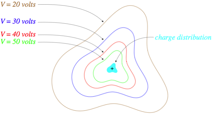
With a positive source charge, the field lines are pointing outward, which is indeed pointing from higher potential to lower potential, but there is something more specific that we can conclude about the geometric relationship of the field and potential. When we follow a path that remains on an equipotential, the potential never changes, so if we traverse such a path from position A to position B, we find:
VA−VB=0=B∫A→E⋅→dl
Certainly the electric field is not zero everywhere we go, and the distance we travel isn't zero, so how can this integral come out to be zero? Maybe parts of it cancel other parts? No, because it happens on every single path we take, between any two points, so long as that path stays on an equipotential. The answer is that the only way this integral can be zero is if at every point on the equipotential, the electric field is perpendicular to →dl. In other words:
The electric field is perpendicular to equipotential surfaces everywhere.
That electric fields are perpendicular to equipotential surfaces sounds very familiar. We said the same thing about conducting surfaces for electrostatics. Indeed, we immediately conclude that for electrostatics:
Conductors are equipotentials.
Note that this statement goes beyond just the surface of the conductor. We know that inside the metal of the conductor there is no electric field, so as we go from the surface of the conductor into the metal, the electric potential can't be changing (electric fields come from changes of electric potential), so the electric potential is the same everywhere in the conductor.
When we are provided with several equipotential surfaces as we are here, we can conclude more about the electric field than just its direction. The gradient operation measures a directional rate of change. This means that if every equipotential surface shown is separated by the same number of volts (as in the diagram above), then the regions where those surfaces are closest together is where they are changing the fastest, which means that the magnitude of the electric field is greatest there.
Example 2.2.2
A charged particle travels through an electric field whose equipotential surfaces are shown in the diagram. The only force experienced by the charge is due to this field. The charge is moving slower at point A than it is at point B.
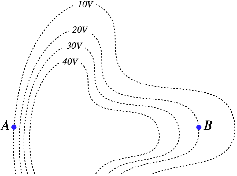
- The charge of the particle is: positive / negative / can't tell
- The magnitude of the charge's acceleration is greater at: point A / point B / can't tell.
- What is the direction of the charge's acceleration at each point?
- Solution
-
a. The particle's kinetic energy increased from point A to point B, which means that its potential energy went down. But its electrostatic potential went up, so since ΔU=qΔV, then ΔU<0 and ΔV>0 means that q<0.
b. The equipotentials all differ by equal voltages, so those that are closer together indicate a region where the electric field is stronger. The field is therefore stronger at point A, which means it experiences a greater net force there than it does at point B.
c. The force due to the electric field must be parallel to the electric field, which must be perpendicular to the equipotential surface. So the forces at points A and B must be either to the left or to the right, but can we tell which way? The field points from higher potential to lower potential, so at point A it points left, and at point B is points right. The charge is negative, so the forces are opposite to the electric field directions. The particle accelerates to the right at point A and to the left at point B.