5.5: Maxwell's Equations

Ampére's Law is Broken

As far as the EM theory had come, a 19th-century Scottish physicist named James Clerk Maxwell felt something had to be missing. To get an idea of what was nagging him, consider Ampére’s law. Recall we said that it only worked for closed loops and infinitely-long wires, because the current had to pierce a surface bounded by the Ampérian circuit. Maxwell felt that there had to be some way to modify Ampére’s law to take care of this shortcoming, and came up with the following thought experiment.

Suppose we have a long-straight wire with a current in it. We can employ Ampére's law for this situation, because if we construct an Ampérian circuit around this wire, every surface – whatever its shape – that is bounded by that closed path must be pierced by that wire. Now suppose the wire includes a single capacitor. Now it is possible to construct a surface bounded by the Ampérian circuit such that the current does not pierce it. Maxwell felt that maybe maybe Ampére's law could be modified such that surfaces not pierced by the current can also be related to the line integral of the magnetic field around the same circuit.

Figure 5.5.1 – Maxwell's Extension of Ampére's law

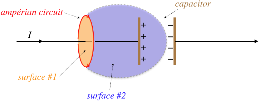
The current piercing surface #1 can be expressed in a manner that transports (or "displaces") the calculation over to the capacitor's electric field. The current passing through surface #1 is the rate at which the charge is building up on the capacitor plate, and this is related to the rate at which the field between the two capacitor plates is growing. Specifically:

\[\left.\begin{array}{l} I=\dfrac{dQ}{dt} \\ \left|\overrightarrow E\right| = \dfrac{\sigma}{\epsilon_o}=\dfrac{Q}{\epsilon_oA} \end{array}\right\} \;\;\;I = \dfrac{d}{dt}\left(\epsilon_o\left|\overrightarrow E\right|A\right) = \epsilon_o\dfrac{d}{dt}\int\limits_{\text{surface #2}}\overrightarrow E \cdot d\overrightarrow A\]

The time rate of change of the electric field flux which accounts for the enclosed current for a surface that is displaced was called the displacement current by Maxwell. It accounts for the fact that while charge does not pass through a particular surface over time, an equivalent about of "current" in the form of increasing (or decreasing) electric field flux takes its place. So in general, in cases where there is both a current piercing a surface and a change in the electric flux through that surface, the line integral of the magnetic field around a closed path that borders that surface is:

\[\oint\overrightarrow B\cdot \overrightarrow {dl} = \mu_o\left(I_{moving\;charge} + I_{displacement}\right) = \mu_oI_{encl} + \mu_o\epsilon_o\dfrac{d}{dt}\int\overrightarrow E \cdot d\overrightarrow A\]

This is Ampére's law modified with Maxwell's displacement current in integral form. We found earlier that Ampére's law could be written in local (differential) form using Stoke's theorem, and since the integral of the electric field flux is over a surface bounded by the same closed path, we can include the second term in this equation:

\[\oint\overrightarrow B\cdot \overrightarrow {dl} = \int \left(\overrightarrow \nabla \times \overrightarrow B\right)\cdot d\overrightarrow A = \mu_o\int \overrightarrow J\cdot d\overrightarrow A + \mu_o\epsilon_o\dfrac{d}{dt} \int\overrightarrow E\cdot d\overrightarrow A\;\;\;\Rightarrow\;\;\; \overrightarrow \nabla \times \overrightarrow B = \mu_o \overrightarrow J+\mu_o\epsilon_o\dfrac{d}{dt}\overrightarrow E\]

Notice that in fact we will get a nonzero magnetic field line integral even if there is no moving charge, if there is a time-varying electric field present. What Maxwell had discovered was, not only did Faraday's law tell us that a time-varying magnetic field causes an electric field to circulate around it, but it worked in the other direction as well: a time-varying electric field gives rise to a magnetic field as well.

Summary of Field Equations

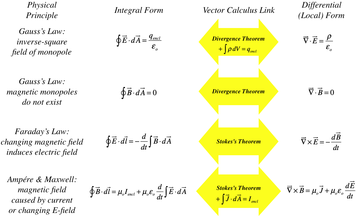
We can now put all of the field equations together, in both integral and local form, to construct a complete theory of electromagnetism. It is summarized in four equations, now known as Maxwell's equations:

Figure 5.5.2 – Maxwell's Equations

Charge Conservation

Electric charge conservation is a fundamental element of the theory of electromagnetism, which we first addressed at the end of Section 3.1, culminating in Equation 3.1.8. Electric charges as sources of both fields are included in Maxwell's equations, so it is absolutely essential that Maxwell's equations be consistent with charge conservation. Thanks to MAxwell's contribution, charge conservation can be derived from the field equations. To see this, consider the identity we have mentioned previously – that the divergence of the curl of any vector field vanishes. Applying this identity to the Ampére/Maxwell equation gives:

\[0 = \overrightarrow \nabla \cdot \left(\overrightarrow \nabla \times \overrightarrow B\right) = \mu_o \overrightarrow \nabla \cdot \overrightarrow J + \mu_o \epsilon_o \overrightarrow \nabla \cdot \dfrac{d\overrightarrow E}{dt} = \overrightarrow \nabla \cdot \overrightarrow J + \dfrac{d}{dt}\left(\epsilon_o \overrightarrow \nabla \cdot \overrightarrow E\right) \]

Now applying the local form of Gauss's law for electric fields to the last term gives the continuity equation (Equation 3.1.8), which expresses charge conservation:

\[0 = \overrightarrow \nabla \cdot \overrightarrow J + \dfrac{d\rho}{dt}\]

So essentially charge conservation is "baked into" the field equations. The field equations give a complete accounting of how fields are generated from conserved electric charge (and its motion), and how the two types of field (electric and magnetic) are generated from each other. What they do not provide is how electric charge is affected by the fields, so we need to add–in the Lorentz force (Equation 4.1.6) to complete the theory:

\[\overrightarrow F = q\left(\overrightarrow E + \overrightarrow v \times \overrightarrow B\right)\]

It turns out that rather than provide the Lorentz force, the interactions of charges with fields can be obtained by knowing the energy densities of the fields, in a manner similar to deriving force from the gradient of potential energy. That is, the theory is also complete if instead of the Lorentz force, one knows:

\[U_{EM} = \frac{1}{2}\epsilon_oE^2+\frac{1}{2\mu_o}B^2\]