
4.1: Magnetic Force


- Last updated
- Aug 12, 2024
- Save as PDF

( \newcommand{\kernel}{\mathrm{null}\,}\)
Forces on Moving Charged Particles
If we run currents through two parallel wires, something unexpected happens – the wires exert forces on each other! One might be inclined at first to explain this by claiming that putting currents through the wires puts electric charge into them, and that the electric charges are exerting electrical forces on each other. But this is not correct. Current is simply a steady flow of charge – there isn't any charge built-up in the wire. For every electron that enters the wire, a corresponding electron exits it.
So the force must have something to do with the motion of the charges. After further experimentation, we find that if we place a stationary net charge near a conducting wire with current, there is no force between them. So apparently there must be motion for both sets of charges in order to exhibit this force.
While this force involves electric charge, it clearly is not electrical in nature. That is, it is altogether different from the Coulomb force. We therefore give it a different name... We call it the magnetic force. Like the electric force, we will explain it in terms of a vector field. And as with the electric force, this will require the two-step theory of first explaining how a charge acts as a source for the field, and then how another charge reacts to being in the presence of a field. We are going to hold off on the first step for now, and focus on the second step, which means we will just start with a magnetic field (without worrying about how it got there), and discuss how the field exerts a force on the moving charge.
We will approach this topic as if we were performing experiments to extract the information we want. Here is a list of our observations from these experiments:
- The strength of the magnetic force on a charge is proportional to the magnetic field through which the charge is moving – This is not surprising, as it was also true for the electric force and field, but more to the point, it really is a result of our definition of magnetic field.
|→FB|∝|→B|
[Note: The traditional variable for magnetic field is B.]
- The strength of the magnetic force on a charge is proportional to the magnitude of the charge – Again, not surprising.
|→FB|∝q|→B|
- The strength of the magnetic force on a charge is proportional to the speed at which the charge is moving though the field – This was mentioned above, and it is the first divergence form the electrical case.
|→FB|∝q|→v||→B|
- The strength of the magnetic force on a charge varies depending upon the relative directions of the magnetic field and the charge's velocity vector – Now this is new! Specifically, we find that the force is zero if the charge happens to be moving parallel to the field, and is its strongest when the field and velocity are perpendicular to each other. Further experimentation reveals that the strength of the force is proportional to the sine of the angle between the field and velocity vectors.
|→FB|∝q|→v||→B|sinθ
- The direction of the magnetic force is perpendicular to both the direction of the velocity and the direction of the magnetic field – This is quite different from the electric case, for which the direction of the force and the field are always in the same or opposite directions.
Perhaps the reader has put together all the puzzle pieces to get to the final expression of the magnetic force on moving point charge:
→FB=q→v×→B
The figure below shows the relationship of the velocity, field, and force vectors. It should be noted that the symbols ⊙ and ⊗ will start playing common roles in diagrams from here on, and they represent the directions "out of the page" and "into the page," respectively. It is also important to note that like the case of the electric force, a negatively-charged particle experiences a magnetic force in the opposite direction of a positively-charged particle under the same conditions.
Figure 4.1.1 – Magnetic Force Direction from Velocity and Field Directions
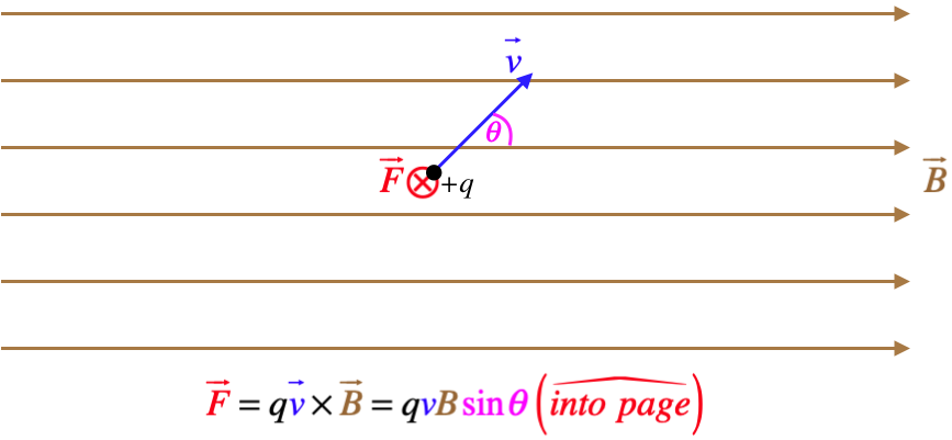
[For a review of the proper use of vector ("cross") products, including the right-hand-rule for determining direction in space, see Section 1.2 of the Physics 9A LibreText.]
There's no reason that electric and magnetic fields can't coexist in the same space. When they do, the force on the point charge is the vector sum of the two forces. The combination (often referred to as the Lorentz force) is therefore:
Before moving on, we should say a word about units. For the equation given above to have proper units, the untis for magnetic field must be force divided by charge-times-velocity. Given how many different names we have for various units, we can of course express this many ways, but once again we will give this quantity its own name:
[B]=[F][q][v]=NC⋅ms=NA⋅m≡T("Tesla")
It turns out that a magnetic field with a magnitude of 1T is quite strong. It is not beyond common experience (neodymium bar magnets get to this strength), but more commonly encountered magnetic fields (such as that of the Earth, or a compass needle) are significantly less, and it is more common to see these field strengths described in units of Gauss (G), which the simply one ten-thousandth of a Tesla.
Charge Motion in a Magnetic Field
A charge within a magnetic field that is subject to no other forces other than the magnetic force, follows a motion with a very interesting property. The magnetic force only acts perpendicular to the direction of motion, which means the charge can never speed up. Such a force can only change the direction of motion. This should be clear from basic vector mathematics, but it can perhaps be more easily understood in terms of energy. If the force is always perpendicular to the direction that the particle is moving, then this force can never do any work, which means it can never cause a change in the particle's kinetic energy.
Let's consider a simple case of a charged particle that moves in a plane that is perpendicular to a uniform magnetic field. This charge would experience a force that never changes magnitude (because the charge remains unchanged, the field is uniform, the direction of the velocity is always at right angles to the field, and as we stated above, it can't speed up. This constant-magnitude force is also always perpendicular to the motion of the particle. These two conditions on the force (constant magnitude and always at right-angles to the motion) sound very familiar – these are the conditions for circular motion! Sure enough, such a particle would move in a closed circle. We can use Newton's 2nd law and what we know about centripetal acceleration to put the magnetic force together with the kinematic details of this particle's motion.
Figure 4.1.2 – Charge Moving in a Plane Perpendicular to a Magnetic Field
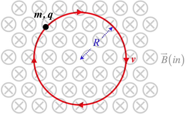
[Note: Is the charge in the figure above positive or negative?]
Ignoring the sign of q (i.e. treating it as an absolute value) we get:
→F=m→ac⇒qvBsin90o=mω2R⇒ω=qmB
The angular speed of the particle depends only upon its charge, its mass, and the magnetic field strength.
Okay, so what if the particle is not moving in this plane? Suppose it has a component of velocity into or out of this plane. Well, this component will be parallel to the magnetic field, and therefore will not contribute to the force on the particle. The components of the velocity in the plane perpendicular to the field still have the same effect. The result is that the particle's motion parallel to the field is totally unaffected, while it moves in a circle in the plane perpendicular to the field. That is, the particle follows a helical path.
Forces on Current-Carrying Wires
We have a vector equation describing the force on a point charge moving through a field, and now we would like to extend this result to currents flowing through conductors in a magnetic field. To do this, we use a common chain-rule trick to relate current through a short length of wire to a moving charge:
I=dqdt=dqdldldt⇒Idl=dqdldt=dqv
If we take into account the direction of the current flow through dl and the velocity, we have the vector version of the contribution of a small segment of current, and we can plug it into the force equation:
I→dl=dq→v⇒d→F=dq→v×→B=I→dl×→B
Figure 4.1.1 only needs to be altered slightly to depict this situation – the wire may be curved, but a tiny segment of it behaves like the point charge.
Figure 4.1.3 – Force on a Tiny Segment of a Current-Carrying Wire
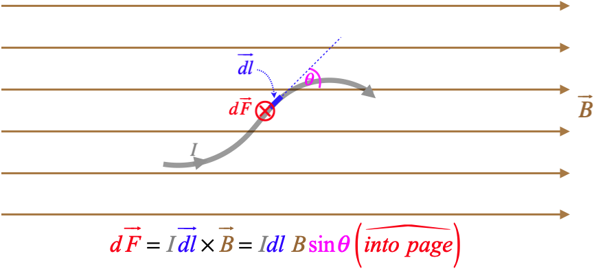
If the total force on a length of wire is desired, all the infinitesimal contributions to force need to be integrated. This can present a challenge is the wire is not straight, since →dl changes direction, or, of course, if the magnetic field changes from one point of the wire to the next. In practice, we frequently deal with straight-line segments in uniform magnetic fields, which yields a simple result for the magnitude (the direction can be determined by the right-hand-rule):
force on straight wire of length L and current I in uniform field B=ILB
We typically deal with currents in closed circuits, so forces on single segments of wire are of limited use. We move on to this more common case next.