
11.6: Electric Dipole
- Page ID
- 80113
\( \newcommand{\vecs}[1]{\overset { \scriptstyle \rightharpoonup} {\mathbf{#1}} } \)
\( \newcommand{\vecd}[1]{\overset{-\!-\!\rightharpoonup}{\vphantom{a}\smash {#1}}} \)
\( \newcommand{\dsum}{\displaystyle\sum\limits} \)
\( \newcommand{\dint}{\displaystyle\int\limits} \)
\( \newcommand{\dlim}{\displaystyle\lim\limits} \)
\( \newcommand{\id}{\mathrm{id}}\) \( \newcommand{\Span}{\mathrm{span}}\)
( \newcommand{\kernel}{\mathrm{null}\,}\) \( \newcommand{\range}{\mathrm{range}\,}\)
\( \newcommand{\RealPart}{\mathrm{Re}}\) \( \newcommand{\ImaginaryPart}{\mathrm{Im}}\)
\( \newcommand{\Argument}{\mathrm{Arg}}\) \( \newcommand{\norm}[1]{\| #1 \|}\)
\( \newcommand{\inner}[2]{\langle #1, #2 \rangle}\)
\( \newcommand{\Span}{\mathrm{span}}\)
\( \newcommand{\id}{\mathrm{id}}\)
\( \newcommand{\Span}{\mathrm{span}}\)
\( \newcommand{\kernel}{\mathrm{null}\,}\)
\( \newcommand{\range}{\mathrm{range}\,}\)
\( \newcommand{\RealPart}{\mathrm{Re}}\)
\( \newcommand{\ImaginaryPart}{\mathrm{Im}}\)
\( \newcommand{\Argument}{\mathrm{Arg}}\)
\( \newcommand{\norm}[1]{\| #1 \|}\)
\( \newcommand{\inner}[2]{\langle #1, #2 \rangle}\)
\( \newcommand{\Span}{\mathrm{span}}\) \( \newcommand{\AA}{\unicode[.8,0]{x212B}}\)
\( \newcommand{\vectorA}[1]{\vec{#1}} % arrow\)
\( \newcommand{\vectorAt}[1]{\vec{\text{#1}}} % arrow\)
\( \newcommand{\vectorB}[1]{\overset { \scriptstyle \rightharpoonup} {\mathbf{#1}} } \)
\( \newcommand{\vectorC}[1]{\textbf{#1}} \)
\( \newcommand{\vectorD}[1]{\overrightarrow{#1}} \)
\( \newcommand{\vectorDt}[1]{\overrightarrow{\text{#1}}} \)
\( \newcommand{\vectE}[1]{\overset{-\!-\!\rightharpoonup}{\vphantom{a}\smash{\mathbf {#1}}}} \)
\( \newcommand{\vecs}[1]{\overset { \scriptstyle \rightharpoonup} {\mathbf{#1}} } \)
\(\newcommand{\longvect}{\overrightarrow}\)
\( \newcommand{\vecd}[1]{\overset{-\!-\!\rightharpoonup}{\vphantom{a}\smash {#1}}} \)
\(\newcommand{\avec}{\mathbf a}\) \(\newcommand{\bvec}{\mathbf b}\) \(\newcommand{\cvec}{\mathbf c}\) \(\newcommand{\dvec}{\mathbf d}\) \(\newcommand{\dtil}{\widetilde{\mathbf d}}\) \(\newcommand{\evec}{\mathbf e}\) \(\newcommand{\fvec}{\mathbf f}\) \(\newcommand{\nvec}{\mathbf n}\) \(\newcommand{\pvec}{\mathbf p}\) \(\newcommand{\qvec}{\mathbf q}\) \(\newcommand{\svec}{\mathbf s}\) \(\newcommand{\tvec}{\mathbf t}\) \(\newcommand{\uvec}{\mathbf u}\) \(\newcommand{\vvec}{\mathbf v}\) \(\newcommand{\wvec}{\mathbf w}\) \(\newcommand{\xvec}{\mathbf x}\) \(\newcommand{\yvec}{\mathbf y}\) \(\newcommand{\zvec}{\mathbf z}\) \(\newcommand{\rvec}{\mathbf r}\) \(\newcommand{\mvec}{\mathbf m}\) \(\newcommand{\zerovec}{\mathbf 0}\) \(\newcommand{\onevec}{\mathbf 1}\) \(\newcommand{\real}{\mathbb R}\) \(\newcommand{\twovec}[2]{\left[\begin{array}{r}#1 \\ #2 \end{array}\right]}\) \(\newcommand{\ctwovec}[2]{\left[\begin{array}{c}#1 \\ #2 \end{array}\right]}\) \(\newcommand{\threevec}[3]{\left[\begin{array}{r}#1 \\ #2 \\ #3 \end{array}\right]}\) \(\newcommand{\cthreevec}[3]{\left[\begin{array}{c}#1 \\ #2 \\ #3 \end{array}\right]}\) \(\newcommand{\fourvec}[4]{\left[\begin{array}{r}#1 \\ #2 \\ #3 \\ #4 \end{array}\right]}\) \(\newcommand{\cfourvec}[4]{\left[\begin{array}{c}#1 \\ #2 \\ #3 \\ #4 \end{array}\right]}\) \(\newcommand{\fivevec}[5]{\left[\begin{array}{r}#1 \\ #2 \\ #3 \\ #4 \\ #5 \\ \end{array}\right]}\) \(\newcommand{\cfivevec}[5]{\left[\begin{array}{c}#1 \\ #2 \\ #3 \\ #4 \\ #5 \\ \end{array}\right]}\) \(\newcommand{\mattwo}[4]{\left[\begin{array}{rr}#1 \amp #2 \\ #3 \amp #4 \\ \end{array}\right]}\) \(\newcommand{\laspan}[1]{\text{Span}\{#1\}}\) \(\newcommand{\bcal}{\cal B}\) \(\newcommand{\ccal}{\cal C}\) \(\newcommand{\scal}{\cal S}\) \(\newcommand{\wcal}{\cal W}\) \(\newcommand{\ecal}{\cal E}\) \(\newcommand{\coords}[2]{\left\{#1\right\}_{#2}}\) \(\newcommand{\gray}[1]{\color{gray}{#1}}\) \(\newcommand{\lgray}[1]{\color{lightgray}{#1}}\) \(\newcommand{\rank}{\operatorname{rank}}\) \(\newcommand{\row}{\text{Row}}\) \(\newcommand{\col}{\text{Col}}\) \(\renewcommand{\row}{\text{Row}}\) \(\newcommand{\nul}{\text{Nul}}\) \(\newcommand{\var}{\text{Var}}\) \(\newcommand{\corr}{\text{corr}}\) \(\newcommand{\len}[1]{\left|#1\right|}\) \(\newcommand{\bbar}{\overline{\bvec}}\) \(\newcommand{\bhat}{\widehat{\bvec}}\) \(\newcommand{\bperp}{\bvec^\perp}\) \(\newcommand{\xhat}{\widehat{\xvec}}\) \(\newcommand{\vhat}{\widehat{\vvec}}\) \(\newcommand{\uhat}{\widehat{\uvec}}\) \(\newcommand{\what}{\widehat{\wvec}}\) \(\newcommand{\Sighat}{\widehat{\Sigma}}\) \(\newcommand{\lt}{<}\) \(\newcommand{\gt}{>}\) \(\newcommand{\amp}{&}\) \(\definecolor{fillinmathshade}{gray}{0.9}\)Definition
We know well how to deal with single point charges and an infinite charged plan which generates a simple form of an electric field, but of course physical systems rarely behave in such a simple way. What we are going to look at here is a model for two point charges that are equal in magnitude and opposite in sign. The reason this is such an important package to develop is that it appears so much in nature, in the form of neutrally-charged molecules.
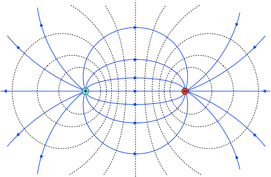
Consider two equal point charges, one positive, and the other negative, that are held rigidly at a fixed separation distance (if you like, you can imagine a tiny rigid rod holding them at fixed relative positions). We have already seen what the field of such a dipole configuration looks like, in Figure 11.3.6. The figure below shows the field lines with equipotential lines included. Since the field lines are now curved, the equipotential circles are also distorted such that they stay perpendicular to the field lines. The density of both the field and the equipotentials is highest near and between the charges, where the additive effect fo the electric fields is greatest with both fields pointing in the same direction.
Figure 11.6.1: Equipotential Surfaces of a Dipole
We could forever treat such a configuration as a combination of two point particles, but it is helpful to package them so that we can treat them as a single entity and not have to go back and recalculate things. To that end, we define a vector quantity known as an electric dipole moment, \(\vec p\), as shown in the figure below.
Figure 11.6.2: Electric Dipole Moment
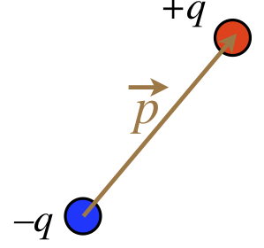
The magnitude of the dipole moment is defined as the product of the absolute value of one of the two charges, multiplied by the distance separating the two charges:
\[\left|\overrightarrow p\right| \equiv q\;d \]
The direction of the dipole moment is that it points from the negative charge to the positive charge.
Alert
Chemists typically define the dipole moment as pointing in the opposite direction. When creating a "package" for later use, how you define it is up to you. We will see that there are compelling reasons (at least in physics applications) for defining it as above.
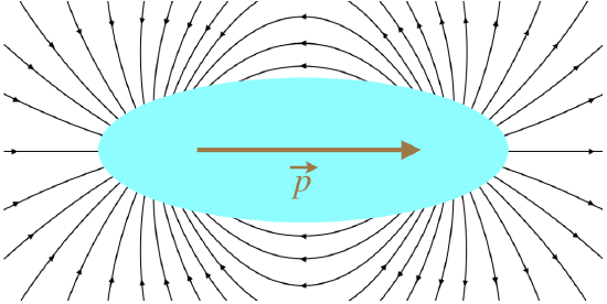
Note that the dipole moment is not the same as the dipole electric field. It may seem funny to even mention this, as these two quantities are not even close to being the same, but it does come up. One place where it gets confusing is that the dipole moment points in the opposite direction as the electric field between the two charges. But as we are forming a package with these two charges, what happens between them is of no consequence. When it comes to the direction of the dipole field, the dipole moment direction makes perfect sense.
Figure 11.6.3: Field of a Dipole
Potential Energy
We consider now the effect that a uniform electric field has on a dipole. Note that while we will be assuming a uniform field, in reality we mean that the amount that the external field changes across the length of the dipole is negligible. Also, as will generally be the case going forward, when we draw a diagram of a uniform field, we will represent it with a set of parallel field lines.
Figure 11.6.4: Dipole in a Uniform Field
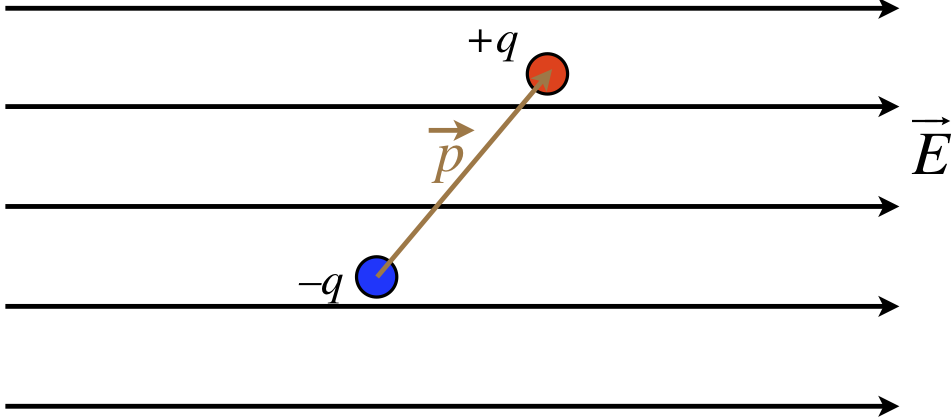
We begin by considering the force on the dipole. Certainly each individual charge feels a new force from the field, but the charges are equal in magnitude, and the forces act in opposite directions, so the net force on it is zero.
Alert
If the field is not uniform, then the dipole can experience a net force! This might seem odd, given that the "package" of two charges is neutrally-charged, but it is an important physical effect to be aware of (we will discuss it in more detail later).
With no net force, the center of mass of the dipole will not accelerate, but there will clearly be a torque exerted on this object with will allow the dipole to rotate about its center of mass. If there is a net torque exerted, there should be a potential energy associated with this interaction. Suppose we release the dipole in the diagram above from rest. Clearly it will begin to rotate, which means it will gain kinetic energy thus some potential energy must be lost.
Figure 11.6.5: Potential Energy Change for a Rotating Dipole in a Uniform Field
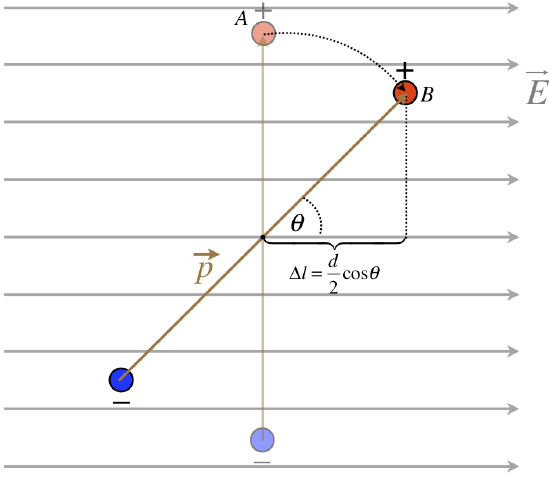
Let us consider the change in potential energy of rotating the dipole by some angle \(\theta\) as shown in the figure above. The horizontal displacement due to this rotation is calculated as \(\Delta l\) in the figure. We have calculated in the previous section that the potential changes linearly in a constant electric field. For a positive charge in the dipole the change in potential energy is then:
\[\Delta PE_p=q\Delta V=-qE\Delta r=-qE\dfrac{d}{2}\cos\theta\]
For the negative change, the horizontal displacement has the same magnitude but a negative sign since the charge is moved in the direction of increasing potential:
\[\Delta PE_n=-q\Delta V=qE\Delta r=-qE\dfrac{d}{2}\cos\theta\]
Combing the two results above, we find that the total change in potential energy is:
\[\Delta PE_p=-(qd)E\cos\theta\]
Note that the energy is a minimum when the dipole moment aligns with the external electric field.