11.3: Electric Field

Last updated

Feb 15, 2023
Save as PDF
- 11.2: Electric Force
- 11.4: Conductors and Infinite Conducting Plates

$\newcommand{\vecs}[1]{\overset { \scriptstyle \rightharpoonup} {\mathbf{#1}} }$

$\newcommand{\vecd}[1]{\overset{-\!-\!\rightharpoonup}{\vphantom{a}\smash {#1}}}$

$\newcommand{\id}{\mathrm{id}}$ $\newcommand{\Span}{\mathrm{span}}$

( \newcommand{\kernel}{\mathrm{null}\,}\) $\newcommand{\range}{\mathrm{range}\,}$

$\newcommand{\RealPart}{\mathrm{Re}}$ $\newcommand{\ImaginaryPart}{\mathrm{Im}}$

$\newcommand{\Argument}{\mathrm{Arg}}$ $\newcommand{\norm}[1]{\| #1 \|}$

$\newcommand{\inner}[2]{\langle #1, #2 \rangle}$

$\newcommand{\Span}{\mathrm{span}}$

$\newcommand{\id}{\mathrm{id}}$

$\newcommand{\Span}{\mathrm{span}}$

$\newcommand{\kernel}{\mathrm{null}\,}$

$\newcommand{\range}{\mathrm{range}\,}$

$\newcommand{\RealPart}{\mathrm{Re}}$

$\newcommand{\ImaginaryPart}{\mathrm{Im}}$

$\newcommand{\Argument}{\mathrm{Arg}}$

$\newcommand{\norm}[1]{\| #1 \|}$

$\newcommand{\inner}[2]{\langle #1, #2 \rangle}$

$\newcommand{\Span}{\mathrm{span}}$ $\newcommand{\AA}{\unicode[.8,0]{x212B}}$

$\newcommand{\vectorA}[1]{\vec{#1}} % arrow$

$\newcommand{\vectorAt}[1]{\vec{\text{#1}}} % arrow$

$\newcommand{\vectorB}[1]{\overset { \scriptstyle \rightharpoonup} {\mathbf{#1}} }$

$\newcommand{\vectorC}[1]{\textbf{#1}}$

$\newcommand{\vectorD}[1]{\overrightarrow{#1}}$

$\newcommand{\vectorDt}[1]{\overrightarrow{\text{#1}}}$

$\newcommand{\vectE}[1]{\overset{-\!-\!\rightharpoonup}{\vphantom{a}\smash{\mathbf {#1}}}}$

$\newcommand{\vecs}[1]{\overset { \scriptstyle \rightharpoonup} {\mathbf{#1}} }$

$\newcommand{\vecd}[1]{\overset{-\!-\!\rightharpoonup}{\vphantom{a}\smash {#1}}}$

$\newcommand{\avec}{\mathbf a}$

$\newcommand{\bvec}{\mathbf b}$

$\newcommand{\cvec}{\mathbf c}$

$\newcommand{\dvec}{\mathbf d}$

$\newcommand{\dtil}{\widetilde{\mathbf d}}$

$\newcommand{\evec}{\mathbf e}$

$\newcommand{\fvec}{\mathbf f}$

$\newcommand{\nvec}{\mathbf n}$

$\newcommand{\pvec}{\mathbf p}$

$\newcommand{\qvec}{\mathbf q}$

$\newcommand{\svec}{\mathbf s}$

$\newcommand{\tvec}{\mathbf t}$

$\newcommand{\uvec}{\mathbf u}$

$\newcommand{\vvec}{\mathbf v}$

$\newcommand{\wvec}{\mathbf w}$

$\newcommand{\xvec}{\mathbf x}$

$\newcommand{\yvec}{\mathbf y}$

$\newcommand{\zvec}{\mathbf z}$

$\newcommand{\rvec}{\mathbf r}$

$\newcommand{\mvec}{\mathbf m}$

$\newcommand{\zerovec}{\mathbf 0}$

$\newcommand{\onevec}{\mathbf 1}$

$\newcommand{\real}{\mathbb R}$

$\newcommand{\twovec}[2]{\left[\begin{array}{r}#1 \\ #2 \end{array}\right]}$

$\newcommand{\ctwovec}[2]{\left[\begin{array}{c}#1 \\ #2 \end{array}\right]}$

$\newcommand{\threevec}[3]{\left[\begin{array}{r}#1 \\ #2 \\ #3 \end{array}\right]}$

$\newcommand{\cthreevec}[3]{\left[\begin{array}{c}#1 \\ #2 \\ #3 \end{array}\right]}$

$\newcommand{\fourvec}[4]{\left[\begin{array}{r}#1 \\ #2 \\ #3 \\ #4 \end{array}\right]}$

$\newcommand{\cfourvec}[4]{\left[\begin{array}{c}#1 \\ #2 \\ #3 \\ #4 \end{array}\right]}$

$\newcommand{\fivevec}[5]{\left[\begin{array}{r}#1 \\ #2 \\ #3 \\ #4 \\ #5 \\ \end{array}\right]}$

$\newcommand{\cfivevec}[5]{\left[\begin{array}{c}#1 \\ #2 \\ #3 \\ #4 \\ #5 \\ \end{array}\right]}$

$\newcommand{\mattwo}[4]{\left[\begin{array}{rr}#1 \amp #2 \\ #3 \amp #4 \\ \end{array}\right]}$

$\newcommand{\laspan}[1]{\text{Span}\{#1\}}$

$\newcommand{\bcal}{\cal B}$

$\newcommand{\ccal}{\cal C}$

$\newcommand{\scal}{\cal S}$

$\newcommand{\wcal}{\cal W}$

$\newcommand{\ecal}{\cal E}$

$\newcommand{\coords}[2]{\left\{#1\right\}_{#2}}$

$\newcommand{\gray}[1]{\color{gray}{#1}}$

$\newcommand{\lgray}[1]{\color{lightgray}{#1}}$

$\newcommand{\rank}{\operatorname{rank}}$

$\newcommand{\row}{\text{Row}}$

$\newcommand{\col}{\text{Col}}$

$\renewcommand{\row}{\text{Row}}$

$\newcommand{\nul}{\text{Nul}}$

$\newcommand{\var}{\text{Var}}$

$\newcommand{\corr}{\text{corr}}$

$\newcommand{\len}[1]{\left|#1\right|}$

$\newcommand{\bbar}{\overline{\bvec}}$

$\newcommand{\bhat}{\widehat{\bvec}}$

$\newcommand{\bperp}{\bvec^\perp}$

$\newcommand{\xhat}{\widehat{\xvec}}$

$\newcommand{\vhat}{\widehat{\vvec}}$

$\newcommand{\uhat}{\widehat{\uvec}}$

$\newcommand{\what}{\widehat{\wvec}}$

$\newcommand{\Sighat}{\widehat{\Sigma}}$

$\newcommand{\lt}{<}$

$\newcommand{\gt}{>}$

$\newcommand{\amp}{&}$

$\definecolor{fillinmathshade}{gray}{0.9}$

Electric Field

In the previous section we made an effort to distinguish the source charge that "generates" the force, and a test charge that "feels" the force. Imagine the source charge is fixed in space, and you move the test charge to another location near the source charge. Then it would will a different force in the new location. In fact, anywhere in space around the source charge, the test charge feels a force. Thus, we can think of the source charge generating a vector quantity everywhere in space, which we will call the electric field. This is consistent with our definition of a vector field from Section 11.1, a vector quantity which has a value everywhere in space. Then, a test charges feel as a force when brought into this field. In other words the source charge generates a vector field around it which can be detected by test charges in a force of a source.

We define this electric field in the following manner. The electric field generated by a source charge $q_{\text{source}}$ is given by:

$\vec E_{q_{\text{source}}}=\dfrac{kq_{\text{source}}}{r^2}\hat r\label{Efield}$

where $r$ is the distance from the source charge to the location where the electric field is calculated. Since the radial unit vector, $\hat r$ , points radially away from the source, if the source charge is positive, $q_{\text{source}}>0$ , then the electric field points in the same direction as $\hat r$ , away from the source. If the charge is negative, $q_{\text{source}}<0$ , then electric field will point in the opposite direction of the radial unit vector, $-\hat r$ , and thus, toward the source charge. Once we have established the electric field that a source charge creates, we can readily calculate the force felt by a test charge, $q_{\text{test}}$ , which is located somewhere in the electric field generated by the source:

$\vec F_{\text{on}q_{\text{test}}\text{by}q_{\text{source}}}=q_{\text{test}}\vec E_{q_{\text{source}}}$

We can see from the above equation that the electric field has units of $N/C$ . The above equation tells us that that if the test charge is positive, the force will point in the same direction as the electric field. For example, we have established that an electric field generated by a positive source charge will point away from it. Thus, if you placed a positive test charge in the electric field, the force it will feel will be in the direction of the electric field, away from the positive source charge. This is consistent with Coulomb's Law of two like charges repelling. Likewise, a negative source charge generates an electric field pointing toward it, so a positive test charge will feel a force in the direction of the field, or toward the negative source charge. Again, this is consistent with two unlike charges being attracted to each other. On the other hand, if the test charge is negative then the force it will feel will be in the opposite direction of the electric field. Thus, a negative test charge will feel a force toward a positive charge which generates an electric field away from it.

We would like to represent this electric field pictorially everywhere in space, as we did for multiple examples of fields in Section 11.1, in particular the vector field map of wind velocity. The electric field a vector field, so we would like to "draw a map" of the vectors around a source charge. Based on Equation $\ref{Efield}$ , the electric field has a fixed magnitude for a given radial distance away from the charge, with vectors pointing away from a positive source. As the radius away from the source charge gets larger, the magnitude of the electric field decreases. Thus, in three-dimensional space there are spherical shells of vectors pointing away from the center. Although a field map is difficult to depict in 3D, we can still have a good representation by depicting the electric field in two dimensions as shown in the left picture below.

Figure 11.3.1: Electric Field Vector and Field Lines for a Positive Charge

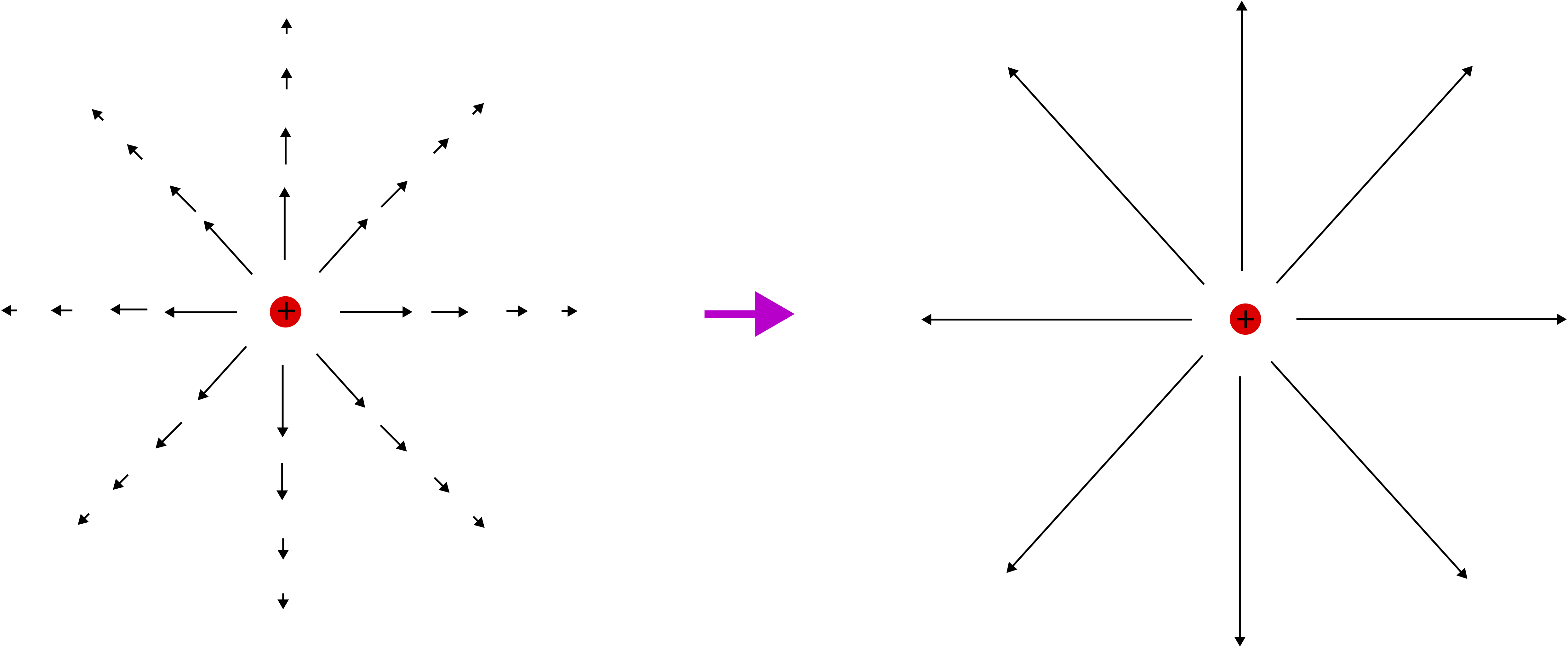
The diagram shows electric field vectors which are symmetric in magnitude at a set radius away from the source charge. They vector arrows are also getting shorter with distance, since the magnitude is decreasing. The electric field is continuous in all of space, so we arbitrary choose a few field vectors to get a good representation of the electric field. In addition, it it difficult to express the relative vector arrows in scale, since the field decreases rapidly as $1/r^2$ , thus the representation above is not scaled very accurately. Instead it is often more convenient to represent the electric field using field lines of field vectors, as shown to the right diagram above. Field lines are "lines" that are tangent to the field vectors. Note, field lines are not the same as field vectors, but they encode some information about field vectors in the following way:

field vectors are tangent to field lines.
the direction of field vectors are indicated by the arrows on the field lines.
the magnitude of the field vectors is indicated by the density of the field lines.

The density of field lines is the number of field lines per unit area. We see that the field lines are most dense near the charge and get less dense as the distance from the charge increase. This is consistent with the magnitude of the field vectors being large near the charge and decreasing as the distance from the charge increases.

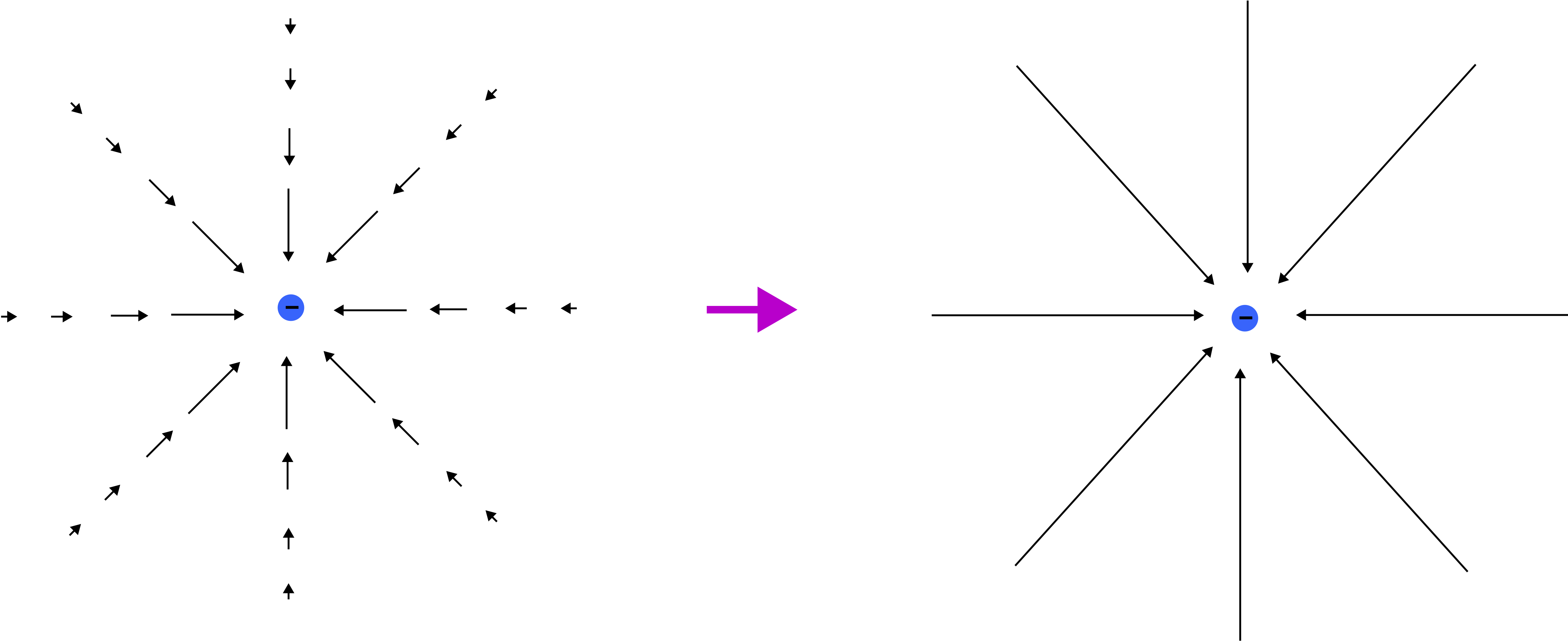
Below is a similar representation for the a negative source charge. Based in Equation $\ref{Efield}$ the field vectors points in the opposite direction of $\hat r$ , or toward the charge. The magnitude is the same as for a positive point charge, large near the charge and decreasing as $1/r^2$ . The field lines representation is also shown for a negative source charge.

Figure 11.3.2: Electric Field Vector and Field Lines for a Negative Charge

The absolute density of field lines show is arbitrary and only displays the relative density with distance. So how would we distinguish the field strength for two separate charges, where one charge is double in magnitude compare to the other? In that case, if you chose eight lines to represent the field lines for the smaller charge, you would draw double the number of lines to express the field lines for the larger charge. Thus, the number of lines drawn to represent the field of some source charge is only relevant when they are compared to other charges.

Superposition

So far we have restricted ourselves to discussing two interacting point charges, such as an electron, a proton, or an ion. In real physical situation, there are often multiple point charges interacting or a charged macroscopic object of some shape interacting with another charged macroscopic object. When this occurs, not only one but multiple charges are exerting an electric force on one particular charge. We have learned from 7B that when multiple charges act on an object, it is the net forces which affects its motion. The net force is a sum of all the forces acting on that object. It is important to remember that since force is a vector, the net force is a vector sum. Thus, to calculate the magnitude of the total force, we first need to add the forces by components and then calculate the magnitude of the total force. To review vector algebra please refer to Section 6.1 of 7B.

We will start with a simple example of a one-dimension vector addition where three charges are located along a line as shown in the figure below. We want to calculate the net force on a positive charge $q_3$ due to the other two charges present, a positive charge $q_1$ and a negative charge $q_2$ . The force on charge 3 by charge 1 is repulsive since both charges are positive, and thus points to the right. The force by charge 2 on charge 3 is attractive, thus it also points to the right. In this case since both forces point in the same direction, you can simply add them to get the total force by both charges, $\vec F_{\text{on 3 by 12}}$ .

Figure 11.3.3: Net Force by Multiple Point Charges

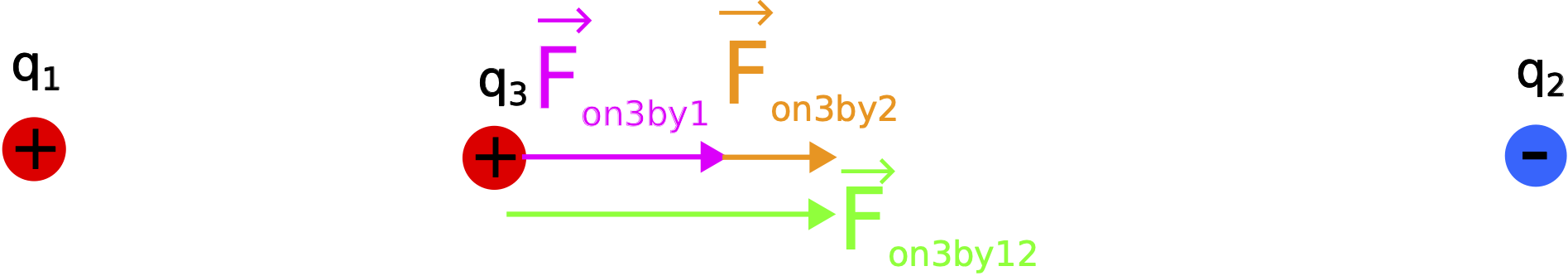
Vector addition in one-dimension is simple. If the two vectors point in the same direction, then you simply add their magnitudes to get the magnitude of the resulting vector, and the direction of that vector is the same as the direction of the two vectors which were added. If the vectors point in opposite directions, then you have to subtract the two magnitudes to get the magnitude of the resulting vector, and the direction of the resulting vector points in the direction of the vector with the larger magnitude. The sum of two vector is zero if the two vectors have the same magnitude but point in opposite direction.

In the figure above, the force by charge 1 is drawn with a bigger magnitude than the force by charge 2. If the two charges, $q_1$ and $q_2$ , have the same magnitude, then this would be certainly the case since $q_1$ is closer in distance than $q_2$ to $q_3$ . However, this does not need to be a general case in this situation, since $q_2$ can have a larger charge magnitude than $q_1$ , such that the difference in charge dominates the difference in distance.

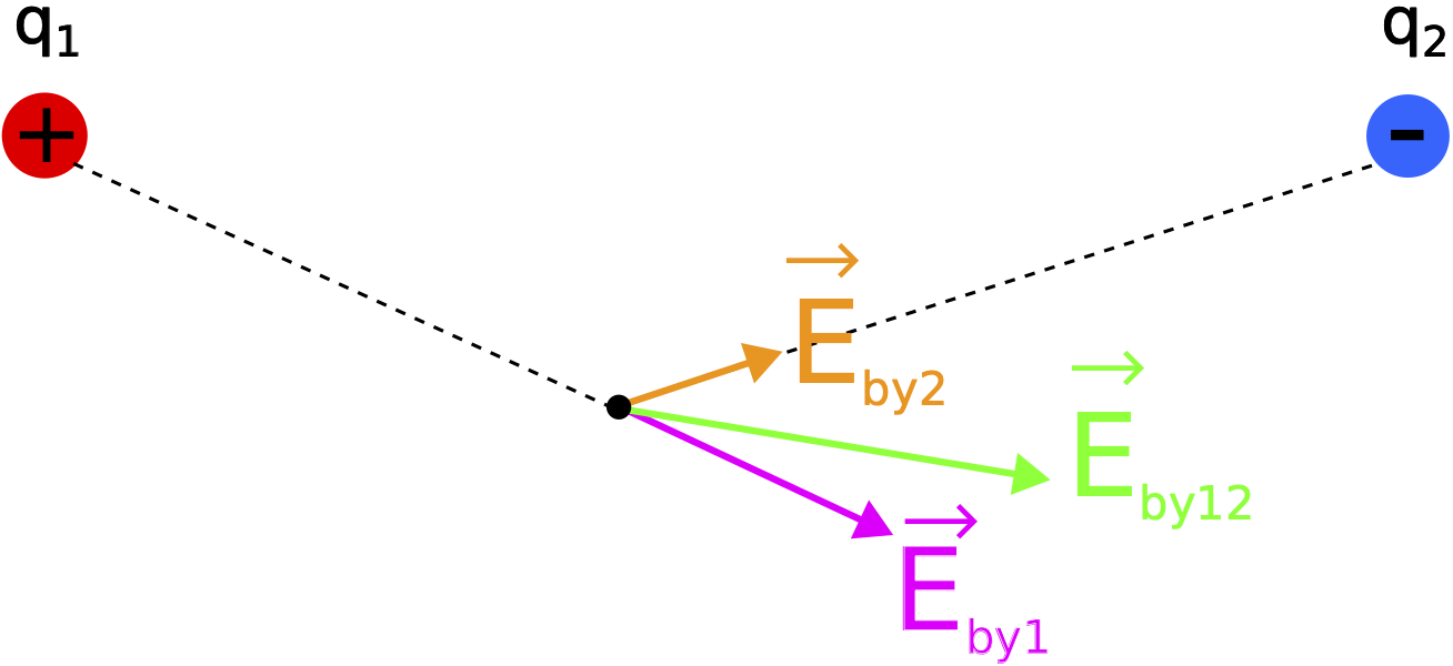
Returning to the electric field, we can describe this scenario as the two charges $q_1$ and $q_2$ being the source of the electric field, while $q_3$ is the test charge that experiences the force due to the presence of this (net) electric field. Thus, we can take the test charge out of the picture for now and map out the electric field at all points in space around the two electric charges. The figure below shows the electric field at a location where the charge $q_3$ was present in Figure 11.3.3. The electric field points away from the positive charge $q_1$ and toward the negative charge $q_2$ . Thus, the net electic field points to the right.

Figure 11.3.4: Net Electric Field by Multiple Point Charges (1D vector addition)

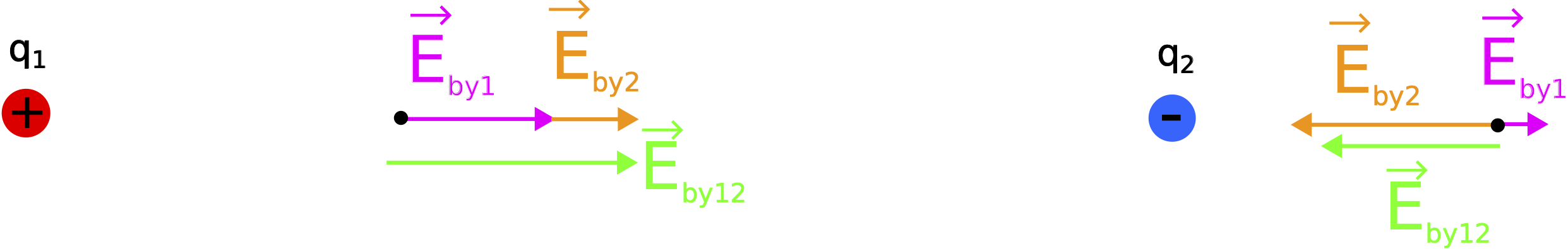
The direction of the net electric field depends on the location relative to the two charges. A second location is shown to the right of the two charges. In this case the electric field by $q_1$ still points to the right (away from the charge) but has a much smaller magnitude since it is further away. (The vector lengths are not drawn to scale here). The field by $q_2$ now points to the left (toward the charge), since the negative charge is now located to the left of this location. It has a bigger magnitude than at the location in between the two charges, since this location is closer to $q_2$ . When adding the two vectors, we subtract the two magnitudes and since the field by $q_2$ is bigger than the field $q_1$ , the net field will point to the left.

Alert

When calculating the electric field be aware of the distinction between magnitude and direction. The direction of the electric field will be dictated by two things: the sign of the charge and the location of the point where the electric field is calculated relative to the charge. The magnitude is then calculated with the absolute value of the charge in Equation $\ref{Efield}$ , since its sign was already considered when determining the direction of the electric field at the specific location where it is measured.

Up to this point we have restricted ourselves to one dimension. However, the field exists everywhere in the three-dimensional space around the two charges. The figure below depicts the total electric field at a location below the line connecting the two charges. In this case since the two charges and the location where the electric field is calculated are not along a straight line, a two-dimensional vector addition is required.

Figure 11.3.5: Net Electric Field by Multiple Point Charges (2D vector addition)

The electric field by $q_1$ points "southeast" away from the positive charge, and the electic field by $q_2$ points "northeast" toward the negative charge. Using the head-to-tail method, we can estimate the direction and the magnitude of the net electric field at that location, as shown in the figure. Mathematically, we can no longer add or subtract the magnitudes of the two electric field. Instead, we need to split each field into components, and then add the components to obtain the net field.

In general, this principle of adding the electric field due to a collection of source charges is known as . Mathematically, the total electric field due to a collection of $N$ source charges can be written as:

$\vec E_{\text{total}}=\sum_{i}^{N}\vec E_i$

We saw in Figures 11.3.1 and 11.3.2 that we can represent electric field vectors with fields lines. The same method applies when mapping the electic field using superposition. We first need to add all the vectors at multiple location and then construct field lines making sure that they are tangent to the net field vectors, have arrows pointing in the direction of the vectors, and have density specifying the field strength at different locations. The figure below depicts the mapping from the individual field vectors of two points charge of opposite charge to the field lines.

Figure 11.3.6: Electric Field Vectors and Field Lines for Two Point Charges

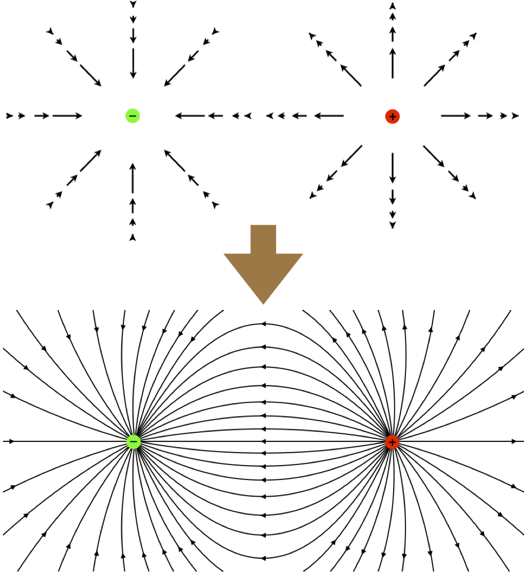
The field lines for this two charge source field are no longer simply straight lines, since the direction of the electric field changes as the position changes. At the location exactly halfway between the two charges the field always points to the left, since the y-components of the fields cancel. However, as the location gets closer to the negative charge for example, the direction of the field is dominated by the negative charge since its magnitude is greater. Thus, the field lines curve toward the negative charges and away from the positive ones. Also, you see the density of the field lines greater closer to the two charges, where the magnitude is greatest. At distances furthest from one of the charges, the field lines start to look a lot like those for an individual point charge, since the effect of the other charge becomes much weaker.

Example $\PageIndex{1}$

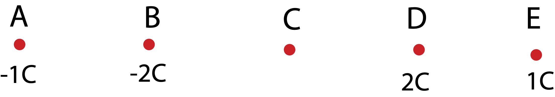
Shown below are equidistant locations marked A-E separated by distance $d=1m$ . The following four charges, 1C, -1C, 2C, and -2C, are placed at locations A, B, D, and E (not necessarily in this order) such that the magnitude of the electric field at location C is maximized and points to the left.

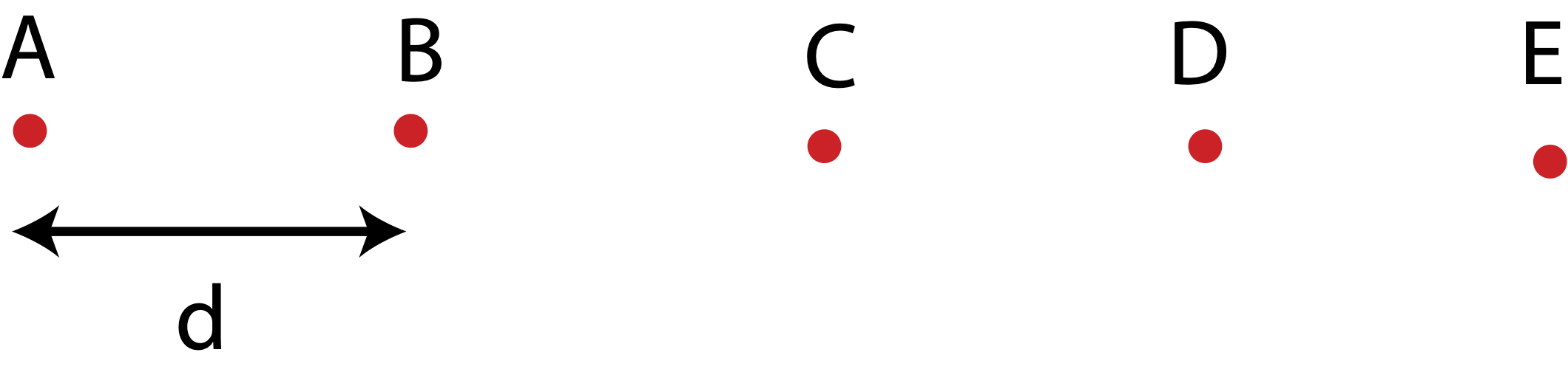
a) Determine where each charge is located.

b) Calculate the magnitude and direction of the force that a -2C charge placed at point C feels due to the presence of the other four charges.

Solution

a) To maximize electric field, the contribution from each charge should additive to the left. So, locations D and E should have positive charges and locations A and B negative ones. You also want to place the charges with the bigger magnitude closer C, since the further position the field is divided by 4 due to double distance. Below is the configuration:

b) The total electric field at location C is:

$\vec E_C=\vec E_A+\vec E_B+\vec E_D+\vec E_E\nonumber$

All the electric fields point to the left at C, toward the negative charges on its left and away from the positive ones on its right. Using the equation for the electric field:

$|\vec E|=\dfrac{kq}{r^2}\nonumber$

and plugging in the values of charges and distances we get:

$\vec E_C=-\dfrac{kC}{4m^2}-\dfrac{2kC}{m^2}-\dfrac{2kC}{m^2}-\dfrac{kC}{4m^2}=-\dfrac{9}{2}\dfrac{kC}{m^2}\nonumber$

The force on a -2C charge placed at C will be to the right, in the opposite direction of the total electric field:

$\vec F_{\text{on -2C}}=(-2C)\vec E_C=9\dfrac{kC}{m^2}=9\cdot 9\times 10^9 \dfrac{Nm^2}{C^2}\dfrac{C}{m^2}=8.1\times 10^{10} N\nonumber$

Example $\PageIndex{2}$

Shown below are 4 identical positive charges located at the corners of a square. The magnitude of the force on charge 1 by charge 4 is $4.0\;\text{N}$ . Find the magnitude of the total force on charge 3 exerted by charges 1, 2, and 4.

Solution

Let the side of the square be distance a. The relevant distances and forces on charge 3 are shown below.

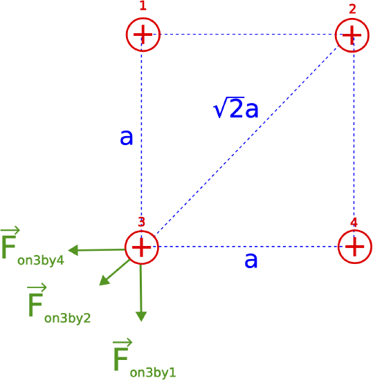
Since the magnitude of the force on charge 1 by charge 4 is 4N, the same as the magnitude on charge 3 by charge 2 is also 4N, since the distance between 1 and 4 is the same as between 2 and 3, and the charges are identical, all positive with the same charge $q$ . Thus, the magnitude of the force on 3 by 2 is given by:

$|\vec F_{\text{on 3 by 2}}|=\dfrac{kq}{2a^2}=4N\nonumber$

The magnitude of the force on 2 by both 1 and 4 are the same since the distance is the same:

$|\vec F_{\text{on 3 by 1}}|=|\vec F_{\text{on 3 by 4}}|=\dfrac{kq}{a^2}\nonumber$

Comparing the two equations above we see that the force by 1 and 4 is double the force by 2. Therefore:

$|\vec F_{\text{on 3 by 1}}|=|\vec F_{\text{on 3 by 4}}|=8N\nonumber$

The direction of the force by 1 is down since the forces are repulsive. In vector form this is written as:

$\vec F_{\text{on 3 by 1}}=(0,-8)N\nonumber$

The direction of the force by 4 is to the left:

$\vec F_{\text{on 3 by 4}}=(-8,0)N\nonumber$

These two vectors combined are:

$\vec F_{\text{on 3 by 1}}+\vec F_{\text{on 3 by 4}}=(-8,-8)N\nonumber$

One way to continue is to break down $\vec F_{\text{on 3 by 2}}$ into components, then add to the sum of the two other forces above, and then find the magnitude. But there is a convenient shortcut when we recognize that the combined vector above will point in the same direction as $\vec F_{\text{on 3 by 2}}$ , thus you can just add their magnitudes (it's now a 1D vector addition) to get the total magnitude of the force:

$|\vec F_{net}|=\sqrt{8^2+8^2}+4=15.3 N$

Search

Text Color

Text Size

Margin Size

Font Type

Electric Field

Superposition

Support Center

How can we help?