
11.5: Electrostatic Potential Energy and Potential
- Page ID
- 78421

\( \newcommand{\vecs}[1]{\overset { \scriptstyle \rightharpoonup} {\mathbf{#1}} } \)
\( \newcommand{\vecd}[1]{\overset{-\!-\!\rightharpoonup}{\vphantom{a}\smash {#1}}} \)
\( \newcommand{\dsum}{\displaystyle\sum\limits} \)
\( \newcommand{\dint}{\displaystyle\int\limits} \)
\( \newcommand{\dlim}{\displaystyle\lim\limits} \)
\( \newcommand{\id}{\mathrm{id}}\) \( \newcommand{\Span}{\mathrm{span}}\)
( \newcommand{\kernel}{\mathrm{null}\,}\) \( \newcommand{\range}{\mathrm{range}\,}\)
\( \newcommand{\RealPart}{\mathrm{Re}}\) \( \newcommand{\ImaginaryPart}{\mathrm{Im}}\)
\( \newcommand{\Argument}{\mathrm{Arg}}\) \( \newcommand{\norm}[1]{\| #1 \|}\)
\( \newcommand{\inner}[2]{\langle #1, #2 \rangle}\)
\( \newcommand{\Span}{\mathrm{span}}\)
\( \newcommand{\id}{\mathrm{id}}\)
\( \newcommand{\Span}{\mathrm{span}}\)
\( \newcommand{\kernel}{\mathrm{null}\,}\)
\( \newcommand{\range}{\mathrm{range}\,}\)
\( \newcommand{\RealPart}{\mathrm{Re}}\)
\( \newcommand{\ImaginaryPart}{\mathrm{Im}}\)
\( \newcommand{\Argument}{\mathrm{Arg}}\)
\( \newcommand{\norm}[1]{\| #1 \|}\)
\( \newcommand{\inner}[2]{\langle #1, #2 \rangle}\)
\( \newcommand{\Span}{\mathrm{span}}\) \( \newcommand{\AA}{\unicode[.8,0]{x212B}}\)
\( \newcommand{\vectorA}[1]{\vec{#1}} % arrow\)
\( \newcommand{\vectorAt}[1]{\vec{\text{#1}}} % arrow\)
\( \newcommand{\vectorB}[1]{\overset { \scriptstyle \rightharpoonup} {\mathbf{#1}} } \)
\( \newcommand{\vectorC}[1]{\textbf{#1}} \)
\( \newcommand{\vectorD}[1]{\overrightarrow{#1}} \)
\( \newcommand{\vectorDt}[1]{\overrightarrow{\text{#1}}} \)
\( \newcommand{\vectE}[1]{\overset{-\!-\!\rightharpoonup}{\vphantom{a}\smash{\mathbf {#1}}}} \)
\( \newcommand{\vecs}[1]{\overset { \scriptstyle \rightharpoonup} {\mathbf{#1}} } \)
\(\newcommand{\longvect}{\overrightarrow}\)
\( \newcommand{\vecd}[1]{\overset{-\!-\!\rightharpoonup}{\vphantom{a}\smash {#1}}} \)
\(\newcommand{\avec}{\mathbf a}\) \(\newcommand{\bvec}{\mathbf b}\) \(\newcommand{\cvec}{\mathbf c}\) \(\newcommand{\dvec}{\mathbf d}\) \(\newcommand{\dtil}{\widetilde{\mathbf d}}\) \(\newcommand{\evec}{\mathbf e}\) \(\newcommand{\fvec}{\mathbf f}\) \(\newcommand{\nvec}{\mathbf n}\) \(\newcommand{\pvec}{\mathbf p}\) \(\newcommand{\qvec}{\mathbf q}\) \(\newcommand{\svec}{\mathbf s}\) \(\newcommand{\tvec}{\mathbf t}\) \(\newcommand{\uvec}{\mathbf u}\) \(\newcommand{\vvec}{\mathbf v}\) \(\newcommand{\wvec}{\mathbf w}\) \(\newcommand{\xvec}{\mathbf x}\) \(\newcommand{\yvec}{\mathbf y}\) \(\newcommand{\zvec}{\mathbf z}\) \(\newcommand{\rvec}{\mathbf r}\) \(\newcommand{\mvec}{\mathbf m}\) \(\newcommand{\zerovec}{\mathbf 0}\) \(\newcommand{\onevec}{\mathbf 1}\) \(\newcommand{\real}{\mathbb R}\) \(\newcommand{\twovec}[2]{\left[\begin{array}{r}#1 \\ #2 \end{array}\right]}\) \(\newcommand{\ctwovec}[2]{\left[\begin{array}{c}#1 \\ #2 \end{array}\right]}\) \(\newcommand{\threevec}[3]{\left[\begin{array}{r}#1 \\ #2 \\ #3 \end{array}\right]}\) \(\newcommand{\cthreevec}[3]{\left[\begin{array}{c}#1 \\ #2 \\ #3 \end{array}\right]}\) \(\newcommand{\fourvec}[4]{\left[\begin{array}{r}#1 \\ #2 \\ #3 \\ #4 \end{array}\right]}\) \(\newcommand{\cfourvec}[4]{\left[\begin{array}{c}#1 \\ #2 \\ #3 \\ #4 \end{array}\right]}\) \(\newcommand{\fivevec}[5]{\left[\begin{array}{r}#1 \\ #2 \\ #3 \\ #4 \\ #5 \\ \end{array}\right]}\) \(\newcommand{\cfivevec}[5]{\left[\begin{array}{c}#1 \\ #2 \\ #3 \\ #4 \\ #5 \\ \end{array}\right]}\) \(\newcommand{\mattwo}[4]{\left[\begin{array}{rr}#1 \amp #2 \\ #3 \amp #4 \\ \end{array}\right]}\) \(\newcommand{\laspan}[1]{\text{Span}\{#1\}}\) \(\newcommand{\bcal}{\cal B}\) \(\newcommand{\ccal}{\cal C}\) \(\newcommand{\scal}{\cal S}\) \(\newcommand{\wcal}{\cal W}\) \(\newcommand{\ecal}{\cal E}\) \(\newcommand{\coords}[2]{\left\{#1\right\}_{#2}}\) \(\newcommand{\gray}[1]{\color{gray}{#1}}\) \(\newcommand{\lgray}[1]{\color{lightgray}{#1}}\) \(\newcommand{\rank}{\operatorname{rank}}\) \(\newcommand{\row}{\text{Row}}\) \(\newcommand{\col}{\text{Col}}\) \(\renewcommand{\row}{\text{Row}}\) \(\newcommand{\nul}{\text{Nul}}\) \(\newcommand{\var}{\text{Var}}\) \(\newcommand{\corr}{\text{corr}}\) \(\newcommand{\len}[1]{\left|#1\right|}\) \(\newcommand{\bbar}{\overline{\bvec}}\) \(\newcommand{\bhat}{\widehat{\bvec}}\) \(\newcommand{\bperp}{\bvec^\perp}\) \(\newcommand{\xhat}{\widehat{\xvec}}\) \(\newcommand{\vhat}{\widehat{\vvec}}\) \(\newcommand{\uhat}{\widehat{\uvec}}\) \(\newcommand{\what}{\widehat{\wvec}}\) \(\newcommand{\Sighat}{\widehat{\Sigma}}\) \(\newcommand{\lt}{<}\) \(\newcommand{\gt}{>}\) \(\newcommand{\amp}{&}\) \(\definecolor{fillinmathshade}{gray}{0.9}\)Electrostatic Potential Energy
Just like forces exist between two objects, the potential energy is always an energy between two objects. In Physics 7A we tied together the idea of potential energy and force. We learned that the force always points in the direction of decreasing potential energy, and the magnitude of the force depends on the rate of change (slope) of potential energy with distance. This is analogous to releasing a ball on a smooth hillside; the ball starts to roll in the direction of the steepest slope of the hill. In two or three dimensions, the force is the derivative of the potential in the direction of “steepest slope". Going back to the topographical map, contour lines with small distances between them indicate steeper hills. Objects placed here would experience higher acceleration (strongest force) down the hill than objects placed elsewhere.
It is worth repeating here the mathematical description that connects force and potential energy. Most generally, when the force is the negative of the gradient of the potential:
\[ \overrightarrow F = -\overrightarrow \nabla PE \label{Fgrad}\]
The gradient operator \(\nabla\) is short-hand for writing:
\[ F_{x} = -\frac{dPE}{dx};~~F_{y} = -\frac{dPE}{dy};~~F_{z} = -\frac{dPE}{dz}\]
where x, y, and z are variables for the three spatial dimensions. We will mostly focus on potential energy between objects where the interaction is spherically symmetric (depends on separation \(r\)), such as between point charges. For these cases, Equation \ref{Fgrad} can be written as:
\[ F(r) = -\frac{dPE(r)}{dr}\label{Fr}\]
where \(F(r)\) is the magnitude of a force which points along the radial component \(\hat r\). To solve for potential energy in terms of force, you can rewrite Equation \ref{Fr} in terms of an integral of force over distance. For a force between two point charges described by Coulomb's Law, the electrostatic potential energy is:
\[PE(r)=-\int F(r)dr=-\int\dfrac{kq_1q_2}{r^2}dr=\dfrac{kq_1q_2}{r}+C\label{PEgen}\]
where the constant \(C\) is some constant, and PE has units of Joules. You can check the equation above by taking the derivative of the potential energy with respect to \(r\) and recovering the equation for the force between two charges. The constant, \(C\), that appears in the potential energy equation should remind us that the absolute value of potential energy is arbitrary. The physically relevant quantity is the change in potential energy when an object moves from one location to another. For gravitational potential energy, the change in height of the object determined the change in potential energy. The actual zero value of the height, and thus potential energy, can chosen at some convenient location. For the Lennard-Jones potential we chose the potential energy to be zero when the two particles were distant and non-interacting. However, this choice of zero did not alter the is the amount of energy required to separate the two particles (break the bond), which is the difference in potential energy between the two particles between far apart and at their equilibrium separation.
Likewise, we can choose a convenient zero value for the electrostatic potential energy. When the two particles are far apart, then electric force becomes very weak. Thus, it makes sense to choose the potential energy to be zero when the two charges are very far apart, \(r\rightarrow\infty\), as was done for the L-J potential. Taking the limit as the separation goes to infinity in Equation \ref{PEgen}, and setting \(PE(r\rightarrow\infty)=0\), we find that \(C=0\). Thus, we write the electrostatic potential energy as:
\[PE(r)=\dfrac{kq_1q_2}{r}\label{PE}\]
Let us think about the connection of the potential energy and force to conceptually understand the equation above. If the two interacting charges are both positive or both negative, then the potential energy is positive. Moving the two charges closer together will result in a positive change in potential energy: \(PE(r)\) increases as \(r\) decreases. The force points in the direction of decreasing potential energy, thus, moving two like charges closer together is moving them in the opposite direction of the force. On the other hand, if we start with two stationary like charges and let them move freely, they will move apart toward larger values of \(r\) in the direction of decreasing potential energy. This is consistent with the force for like charges being repulsive and wanting to push the charges apart. You can also think about this in terms of conservation of energy, if the potential energy decreases, then kinetic energy must increase. Thus, as the two charges repel, then speed up as they separate.
If the two charges have opposite signs, then the potential energy is negative. This means that the potential energy decreases when the two charges move closer together (the potential energy will get more negative). Thus, the two charges will speed up as them come together and their potential energy decreases toward the force which is attractive for two unlike charges.
Another way to think about potential energy is the energy required to bring charges together from infinity (where potential energy is zero). If there are multiple charges, then you need to consider interactions between all the pairs involved. For example, to assemble three charges, \(q_1\), \(q_2\), and \(q_3\), the potential energy is:
\[PE=\dfrac{kq_1q_2}{r_{12}}+\dfrac{kq_1q_3}{r_{13}}+\dfrac{kq_2q_3}{r_{23}}\]
where \(r_{12}\) is the separation between charges 1 and 2, \(r_{13}\) is the separation between charges 1 and 3, and so on.
Electrostatic Potential
In the previous section we defined the electric field, which is a vector field generated by a charge, a collection of source charges, or a macroscopic charged object. Once the electric field is determined, one can compute the force that a test charge feels when it is placed in the electric field. We can define an analogous field related to potential energy. Let us assign a charge or a collection of charges that generates a scalar field defined everywhere in space, which we call the electrostatic potential, V, sometimes referred to as simply electric potential or voltage.Then, we can analyze that amount of potential energy required to to bring a test electric charge to some location in this potential field. For one point source charge, \(q_{\text{source}}\), the electric potential is defined as:
\[V_{q_{\text{source}}}=\dfrac{kq_{\text{source}}}{r}\label{V}\]
The units of the electric potential are joules per coulomb, \(\dfrac{J}{C}\), also known as Volts, V. The amount of potential energy required to bring a test charge, \(q_{\text{test}}\), from infinity to a distance of \(r\) from the source charge is then given by:
\[PE=q_{\text{test}}V_{q_{\text{source}}}\]
Although, there is a direct relationship between force, which is a vector quantity, and energy, the potential energy is a scalar quantity which has no direction. Since the potential energy is a scalar, so is the electric potential based on equation above.
Alert
Possibly the most confusing thing to students new to electrostatics is use of the word "potential" in "electrostatic potential." This name derives from the fact that it is related to electric potential energy, but these quantities are very different, and the reader is advised to keep this in mind.
The same rules of superposition apply to the electric potential as did for the electric field. If there is a collection of charges then the total electric potential generated by these charges is the sum of the electric potentials due to each charge. Except the total electric potential is much easier to calculate since it is a scalar field, thus it is simply a sum of numbers. The only thing that you need to be careful about is the sign of each charge since the potential can be either positive or negative. For \(N\) charges, the total electric potential:
\[V_{\text{tot}}=\sum_{i=1}^{N}\dfrac{kq_i}{r_i}\]
where \(r_i\) is the distance from the location where the voltage is calculated to the charge \(q_i\).
Example \(\PageIndex{1}\)
The figure below shows four charges fixed at corners of a square. Points A, B, D, and E are midway between two neighboring charges and point C is at the center of the square.
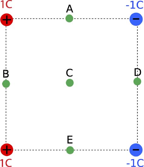
a) At which of the points is the total voltage due to the 4 charges zero?
b) For the locations where the total voltage is not zero, calculate the potential energy of a -2C charge placed at those locations. Leave your answer in terms of the length of a side of the square, \(d\), and the constant \(k\).
- Solution
-
a) The total voltage at each point is the sum of the voltages due to each charge. For each charge:
\[V=\dfrac{kq}{r}\nonumber\]
The four charges have the same magnitude, so we only need to worry about their sign and distance to each location. At point B the two positive charges are closer than the negative charges, so the total voltage will be positive. At point D the two negative charges are closer than the positive charges, so the total voltage will be negative. At points A,C, and E, there is one positive charge and one negative charge the same distance away, so the voltages will cancel at those points.
b) At location B, the distance to each positive charges is:
\[r_p=\dfrac{d}{2}\nonumber\]
We need to use Pythagorean theorem to find the distance to the negative charges:
\[r_n=\sqrt{\Big(\dfrac{d}{2}\Big)^2+d^2}=\dfrac{\sqrt{5}}{2}d\nonumber\]
Thus, we find that the total voltage due to the 4 charges is:
\[V_{B}=\dfrac{4kC}{d}-\dfrac{4kC}{\sqrt{5}d}=2.21\dfrac{kC}{d}\nonumber\]
At location D, the same applies except the negative charges are at the closer distance, and the positive ones are at the further one. Therefore, the total voltage has the same magnitude but opposite sign of the result above:
\[V_{D}=-2.21\dfrac{kC}{d}\nonumber\]
Summary: Force, Field, Potential, and Potential Energy
In the previous section we have established the connection between electric force and field: source charges generate a vector field, and a test charge feels a force in the presence of the field. Likewise, source charges generates a potential scalar field, and a test charge placed in this field will have some potential energy. Mathematically, these relationships are given in the following way:
\[\vec F=q_{\text{test}}\vec E_{q_{\text{source}}}\]
\[PE=q_{\text{test}}V_{q_{\text{source}}}\]
The quantities on the left side of the two equations above are depend on both the source and the test charge since they describe the interaction. The quantities on the right side of the equation that multiply the test charge solely depend on the source charges.
We also used the previously learned relationship between force and potential energy, which leads directly to a new relationship between electric field and electric potential. For a point charge these are:
\[ \vec F = -\dfrac{dPE}{dr}\hat r \]
\[ \vec E = -\dfrac{dV}{dr}\hat r \label{EV}\]
The second equation comes directly from the first by dividing each side of the first equation by test charge: dividing the left side of the equation by \(q_{\text{test}}\) we get the electric field, and dividing the right side of the equation by \(q_{\text{test}}\) we get the electric potential. From the equation above we conclude that electric field points in the direction of decreasing potential, since force points in the direction of decreasing potential energy.
Here is the summary of the important concepts to keep in mind while working with these four quantities:
- An electric field is generated by a source charge or a collection of source charges.
- An electric field points away from a positive charge and toward a negative charge.
- For a collection of source charges, the total electric field at some location is computed by adding the electric field vectors generated by each charge.
- A positive test charge feels a force in the same direction as the electric field, and a negative test charge feels a force in the opposite direction of the electric field.
- An electric potential is generated by a source charge or a collection of source charges.
- An electric potential is always positive and decreases away from a positive charge, and is always negative and increases away from a negative charge.
- For a collection of source charges, the total electric potential at some location is computed by adding the electric potentials generated by each charge.
- A positive test charge decreases in potential energy as it moves toward decreasing electric potential, and a negative test charge increases in potential energy as it moves toward decreasing electric potential.
- Electric field points in the direction of decreasing electric potential.
- Electric force points in the direction of decreasing potential energy.
Alert
The relation between field and potential is often misunderstood, in yet another incarnation of confusing a quantity with a change in that quantity (like mistaking acceleration with velocity. Just as zero instantaneous velocity does not mean the acceleration is zero, a zero potential at a point in space does not mean that the field there is zero. Indeed, we can define the potential to be zero anywhere, no matter what the field is! It is the rate of change of the potential that determines the field, not the value of the potential. It is also important to remember that we are relating a vector quantity to a scalar one. The electric potential may be constant and not changing, which only implies that the field is zero along the direction where the potential is not changing. But the field can still be non-zero since it may have components in other directions.
The figure below demonstrates some of these common misconceptions in connecting the electric field and potential. The scenario on the left shows a positive test charge which is moved along the line in between two identical positive source charges. The situation on the right shows a positive test charge that is moved between a positive and a negative source charge of equal magnitude.
Figure 11.5.1: Field and Potential For Two Point Charges
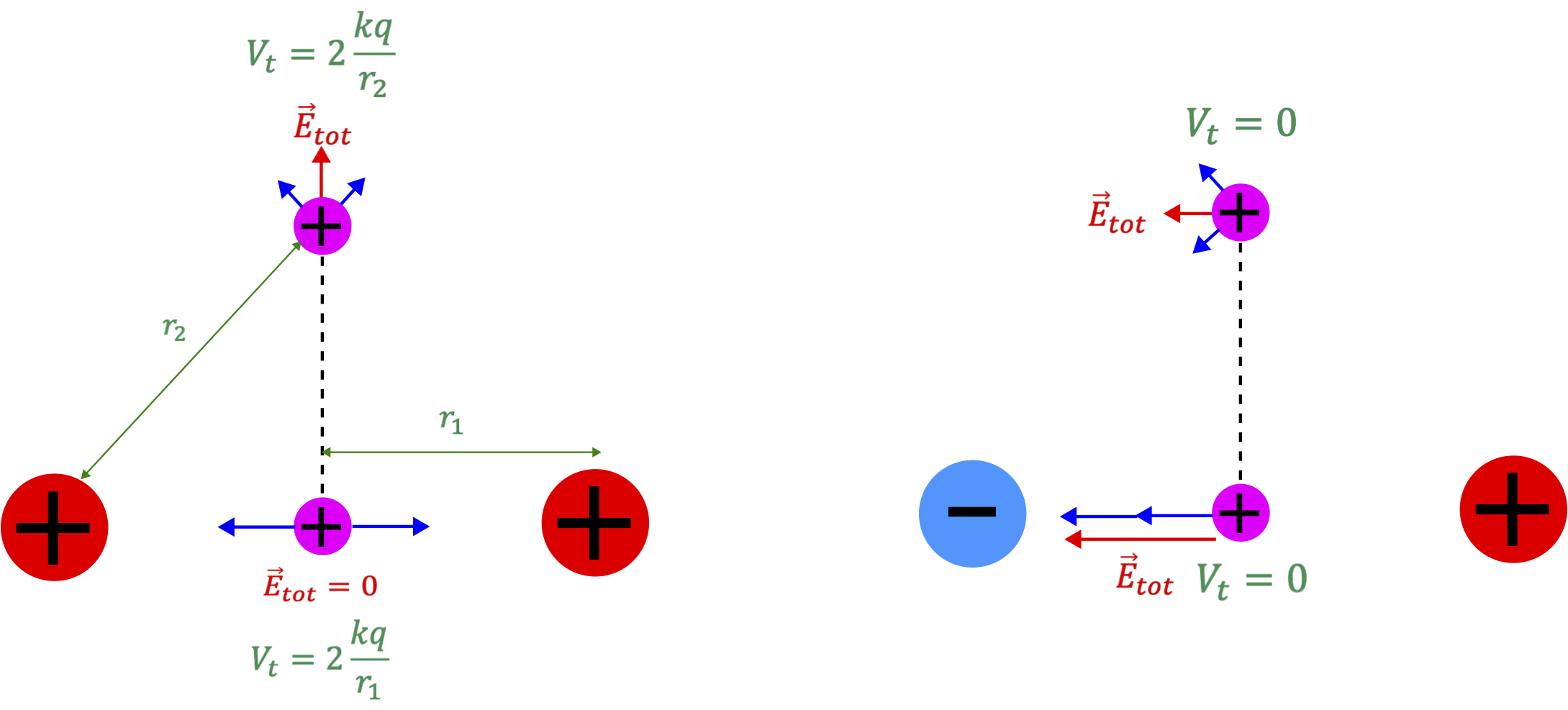
In the scenario on the left, the force is zero on the test charge when it is right in between the two charges. The total electric field is zero at that location, since the electric fields from each source charge are equal in magnitude but opposite in direction. However, this does not imply that the potential is zero at that location. In fact, the total potential has an equal positive contribution from each charge, resulting in a total potential of \(V_t=2\dfrac{kq}{r_1}\). You may think how can the electric field be zero and the potential be non-zero based on their relationship given by Equation \ref{EV}. The reason that the field goes to zero, is that at the central location the potential is not changing for very small displacements along the central line. Right above and right below the central location the distance to both charges is the same. Thus, the potential is constant for a small vertical displacement through the center resulting is zero rate of change of the electric potential, and thus zero electric field at the center. As the test charge moves up and away from the two charges, you can see that there is a net vertical component to the total electic field, so the charge will feel a vertical force. The electric potential decreases in that direction since \(r_2>r_1\), which is consistent with the electric field pointing in the direction of the decreasing potential.
The scenario on the right is another interesting situation, since the electric potential is zero along the line separating the two charges. This is the case since the distance to each charge is the same, but one is positive and the other is negative of equal magnitude, so the total potential adds to zero. However, this does not necessarily mean that the electric field is zero along that line. In fact as shown in the figure, there electric field is non-zero everywhere along that line and points to left, toward the negative charge and away from the positive. At first glance this does not seem to be consistent with Equation \ref{EV} since the potential is not changing, but yet the field is non-zero. However, we need to remember that the field is a vector quantity. Equation \ref{EV} tells us that the field must be zero along the direction where the potential is not changing. This is true for this case, since the field has no vertical component. However, the field can still be non-zero in a direction perpendicular to the central line, as seen in the figure. In fact, if you calculated the potential along the direction of the field, you would discover that it does indeed decrease in that direction since it's getting closer to the negative charge and further from the positive one.
Equipotential Surfaces
In the previous section we describe a useful tool for depicting electric fields using field lines. A similar informative depiction exists for the electric potential. Going back to topographical maps in Section 11.1, we saw that it described a scalar field with lines representing location of constant value of the field (elevation). The elevation difference between neighboring lines was fixed. This means that regions where the contour lines were most dense, where regions where the slope was the largest (elevation changed most rapidly with distance). The opposite was true for regions of low density.
If we want to use a similar representation for electric potential, we will draw curves where the potential is constant, known as equipotential surfaces. Equation \ref{V} tells us that the electric potential is constant along a radius, \(r\), around a point charge. Therefore, equipotential surfaces around point charges will be spherical shells. In a two-dimensional illustration, the surfaces will become circles around the charges.
As for a topographical map where neighboring contour lines were separated by a fixed value of elevation, we want to draw equipotential surfaces separated by a fixed value of potential. Thus, we need to determine how voltage changes with distance in order to know how to space the equipotentials. The figure below is a plot of electric potential as a function of distance for a positive source charge.
Figure 11.5.2: Electric Potential Plot for a Positive Charge
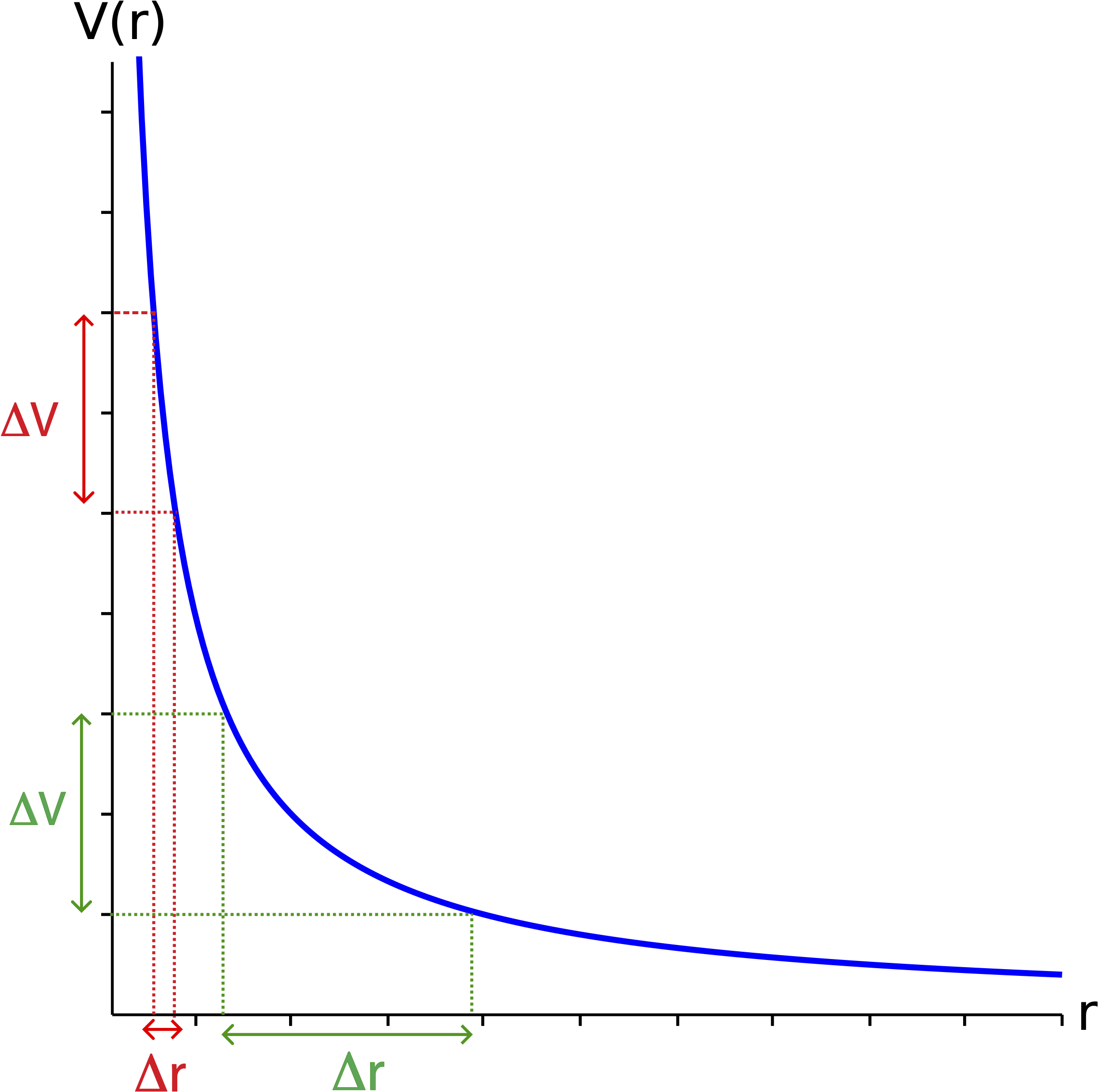
From the plot you can see that for small values of \(r\) (close to the source charge), the voltage changes more rapidly (slope is larger) compared to larger distances from the charge. Therefore, two equipotential surfaces near the charge will be separated by a smaller distance, \(\Delta r\), compared to neighboring equipotential surfaces further from the charge, \(\Delta r\) is bigger for the same \(\Delta V\).
For a positive source charge the electric potential is positive and decreases with distance. For a negative source charge the electric potential is negative and increase with distance. All of these concepts are illustrated in the figure below, together with the field lines for a positive and a negative point charge. As shown the equipotential surfaces get less dense away from the change. The electric potential values are arbitrarily selected to change by 1V, for the sake of demonstrating the sign and change of the potential.
Figure 11.5.3: Equipotential Lines for Point Charges
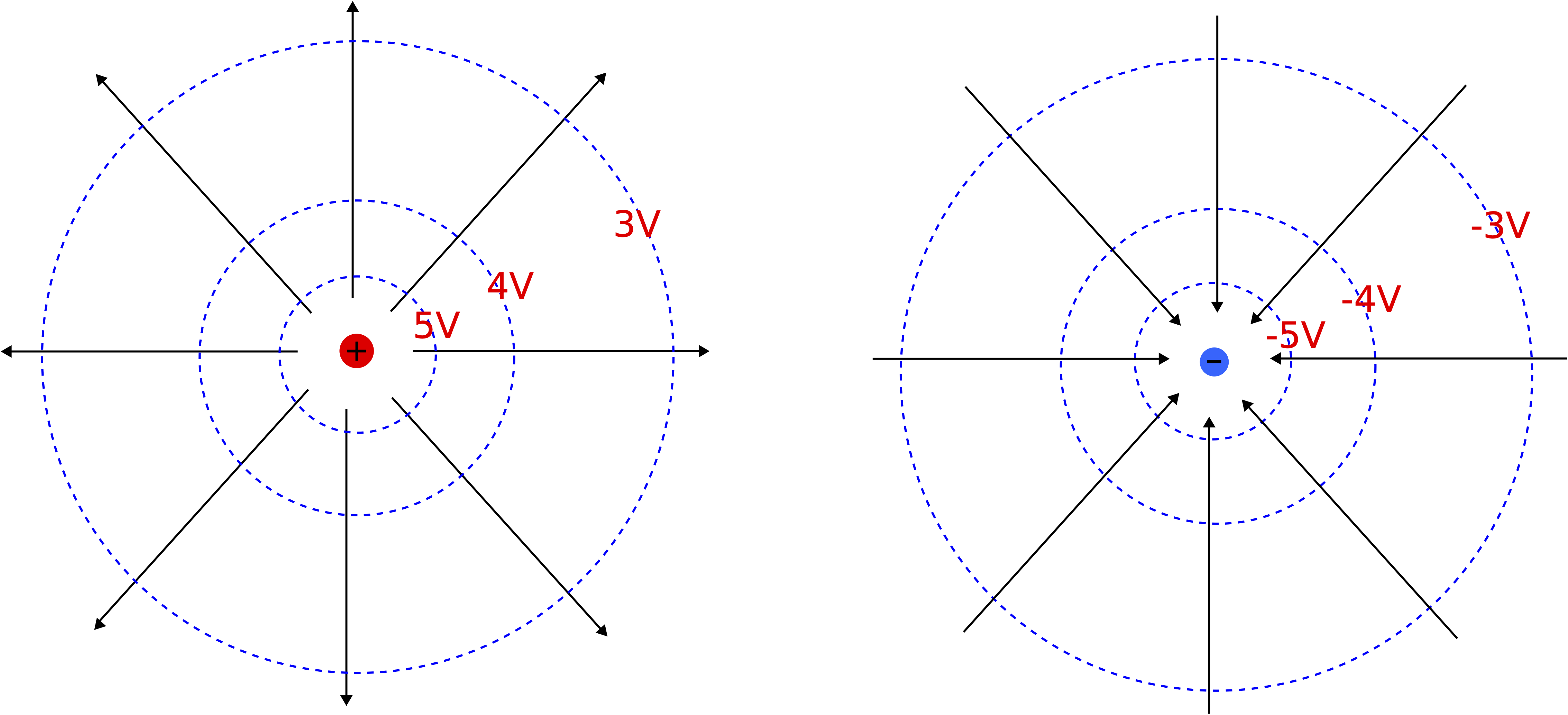
The field lines appear to be perpendicular to the equipotential surfaces and point in the direction of decreasing potential. Since the electric field is the rate of change of the electric potential, when the electric potential is constant the electric field must be zero according to Equation \ref{EV}. Therefore, since equipotentials describe surfaces of constant potential there cannot be any component of the electric field parallel to the equipotential. Therefore, fields lines are always perpendicular to equipotential surfaces. In addition, the density of equipotential lines correlates with the density of field lines. The electric field has the greatest magnitude where the the field lines are most dense. Larger magnitude of electric field, implies larger derivative of voltage with distance according to Equation \ref{EV}. Thus, the equipotential surfaces will be densest where the field lines are most dense.
In the previous section we looked as a special case of a charged infinite conducting plane, where we discovered that the electric field is constant with distance away from the plane. For this scenario Equation \ref{EV} tells us that the electric potential has to be linear with distance in order to result in a constant electric field, since the derivative of a linear function results in a constant. In other words, the change in electric potential linearly depends on the distance away from the plane:
\[\Delta V_{\text{plane}}=-E\Delta r\label{Vplane}\]
Therefore, the equipotential surfaces away from the plane will be equidistant, as shown in the figure below. This is consistent with the fact that the density of the electric field lines is constant, implying that the density of the equipotential surfaces must be constant as well. As previously argued, the equipotential lines are perpendicular to the field lines.
Figure 11.5.4: Equipotential Lines for an Infinite Charged Plane
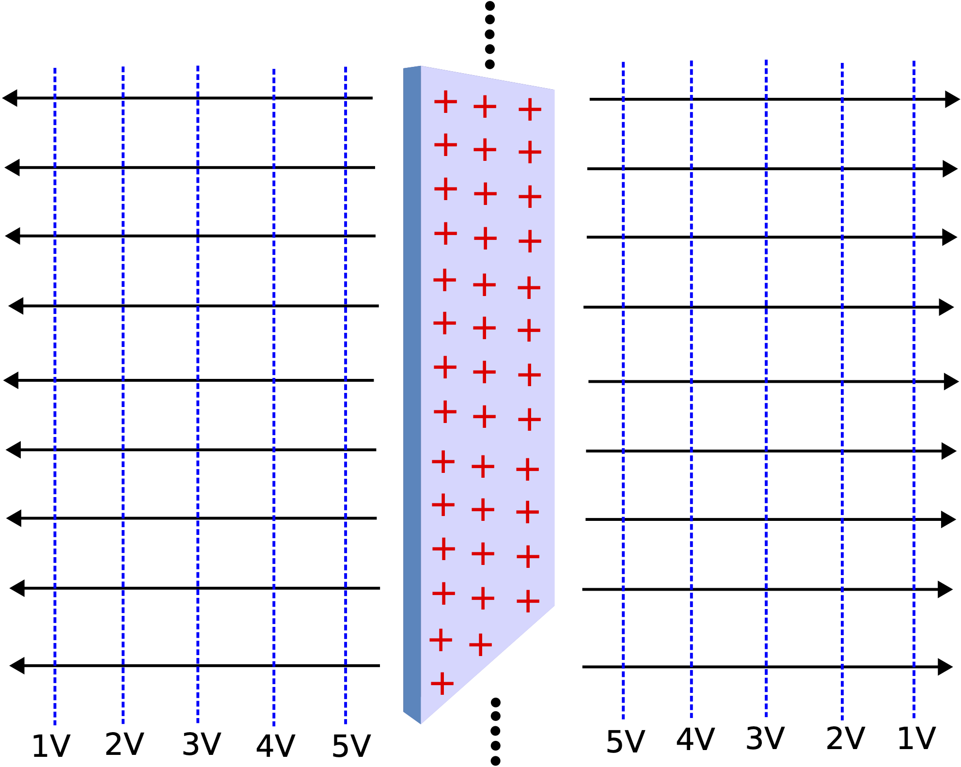
Arbitrary values of the electric potential are assigned in the figure above to stress the potential is positive and decreasing away from a positively charged plane in the direction of the electric field. A positive test charge placed in this field will then will a constant force away from the plane, and its potential energy will decrease as it moves away from the plane. The opposite is true fo a negative test charge, it will feel a force toward the plane, and its potential energy will decrease toward the plane, in the direction of increasing electric potential.
Example \(\PageIndex{2}\)
A charged particle travels through an electric field whose equipotential surfaces are shown in the diagram. The only force experienced by the charge is due to this field. The charge is moving slower at point \(A\) than it is at point \(B\).
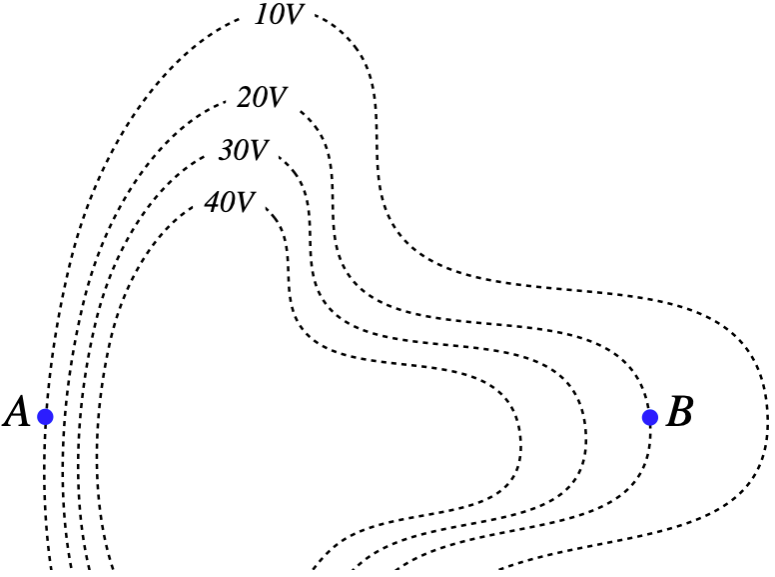
- The charge of the particle is: positive / negative / can't tell
- The magnitude of the charge's acceleration is greater at: point A / point B / can't tell.
- What is the direction of the charge's acceleration at each point?
- Solution
-
a. The particle's kinetic energy increased from point A to point B, which means that its potential energy went down. But its electrostatic potential went up, so since \(\Delta U = q\Delta V\), then \(\Delta U <0\) and \(\Delta V >0\) means that \(q<0\).
b. The equipotentials all differ by equal voltages, so those that are closer together indicate a region where the electric field is stronger. The field is therefore stronger at point A, which means it experiences a greater net force there than it does at point B.
c. The force due to the electric field must be parallel to the electric field, which must be perpendicular to the equipotential surface. So the forces at points A and B must be either to the left or to the right, but can we tell which way? The field points from higher potential to lower potential, so at point A it points left, and at point B is points right. The charge is negative, so the forces are opposite to the electric field directions. The particle accelerates to the right at point A and to the left at point B.
Example \(\PageIndex{3}\)
Shown below are equidistant equipotential horizontal lines due to some source incremented by 4V. The top equipotential line represents 0V. The bottom equipotential line is 6 meters below the top equipotential line and has a lower voltage. Also, located on one of the lines and at the center of a circle is a \(2\times 10^{-9}\;\text{C}\) positive charge. The circle represents locations where test charges are placed in order to determine the forces they would feel.
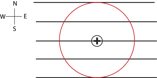
a) Calculate the force that a negative charge with magnitude of \(5\times 10^{-9}\;\text{C}\) feels placed on the circle directly east from the charge in the center. Express the force in terms of magnitude and direction.
b) Calculate the total voltage at the location of the added charge in part a).
c) Calculate the change in potential energy of the negative charge from a) when it moves from directly east to directly south on the circle.
- Solution
-
a) In order to find the net force on the negative test charge, we need to consider the total electric field at the location of the charge due to the source that generated the equipotential lines and due to the positive point charge at the center of the circle.
The electric field due to the equipotential lines is constant since the lines are equally spaced. Its magnitude is:
\[E_{\text{lines}}=\dfrac{\Delta V}{\Delta r}=\dfrac{4\times 4V}{6m}=2.67 \dfrac{V}{m}\nonumber\]
The electric field points in the direction of decreasing voltage, thus, it points South:
\[\vec E_{\text{lines}}=(0,-2.67)\dfrac{N}{m}\nonumber\]
The radius of the circle is 3 m. Thus, the magnitude of electric field 3 m from the positive point charge in the center is:
\[E_q=\dfrac{kq}{r^2}=\dfrac{9\times 10^{9}\dfrac{Nm^2}{C^2}\cdot 2\times 10^{-9} C}{(3m)^2}=2 \dfrac{V}{C}\nonumber\]
The electric field due to the central charge points away from it since it’s positive. Thus, it points East at the location of this charge:
\[\vec E_q=(2,0) \dfrac{V}{m}\nonumber\]
The total electric field is then the sum of the two electric fields above:
\[\vec E_{tot}=\vec E_{\text{lines}}+\vec E_q=(2,-2.67) \dfrac{V}{m}\nonumber\]
The force on the negative charge is:
\[\vec{F}=q\vec E_{tot}=(-5\times 10^{-9} C)(2,-2.67) \dfrac{V}{m}=(-10\times 10^{-9},13.35\times 10^{-9})N\nonumber\]
The magnitude of the force is:
\[|\vec{F}|=\sqrt{(10\times 10^{-9})^2+(13.35\times 10^{-9})^2}=1.67\times 10^{-8}N\nonumber\]
The direction is north of west at an angle of:
\[\theta=\tan^{-1}\dfrac{13.35}{10}=53.16^{\circ}\nonumber\]
b) From the equipotential lines, the voltage of the third line from the top is:
\[V_{\text{lines}}=-2\times 4V=-8V\nonumber\]
From the charge in the center:
\[V_{q}=\dfrac{kq}{r}=\dfrac{9\times 10^{9}\dfrac{Nm^2}{C^2}\cdot 2\times 10^{-9} C}{3m}=6V\nonumber\]
The total voltage at that location is the sum of the two voltages:
\[V_{tot}=V_{\text{lines}}+V_q=-8V+6V=-2V\nonumber\]
c) Since the circle defines an equipotential for the central charge, only contribution to the change of the potential energy are the equipotential lines:
\[\Delta PE=q\Delta V_{\text{lines}}=(-5\times 10^{-9} C)(-8V)=40\times 10^{-9} J\nonumber\]