4.4: Spherical Refractors

Last updated
Save as PDF

Page ID: 18462

$ \newcommand{\vecs}[1]{\overset { \scriptstyle \rightharpoonup} {\mathbf{#1}} } $ $ \newcommand{\vecd}[1]{\overset{-\!-\!\rightharpoonup}{\vphantom{a}\smash {#1}}} $$\newcommand{\id}{\mathrm{id}}$ $ \newcommand{\Span}{\mathrm{span}}$ $ \newcommand{\kernel}{\mathrm{null}\,}$ $ \newcommand{\range}{\mathrm{range}\,}$ $ \newcommand{\RealPart}{\mathrm{Re}}$ $ \newcommand{\ImaginaryPart}{\mathrm{Im}}$ $ \newcommand{\Argument}{\mathrm{Arg}}$ $ \newcommand{\norm}[1]{\| #1 \|}$ $ \newcommand{\inner}[2]{\langle #1, #2 \rangle}$ $ \newcommand{\Span}{\mathrm{span}}$ $\newcommand{\id}{\mathrm{id}}$ $ \newcommand{\Span}{\mathrm{span}}$ $ \newcommand{\kernel}{\mathrm{null}\,}$ $ \newcommand{\range}{\mathrm{range}\,}$ $ \newcommand{\RealPart}{\mathrm{Re}}$ $ \newcommand{\ImaginaryPart}{\mathrm{Im}}$ $ \newcommand{\Argument}{\mathrm{Arg}}$ $ \newcommand{\norm}[1]{\| #1 \|}$ $ \newcommand{\inner}[2]{\langle #1, #2 \rangle}$ $ \newcommand{\Span}{\mathrm{span}}$$\newcommand{\AA}{\unicode[.8,0]{x212B}}$

Spherical Surface Refractions

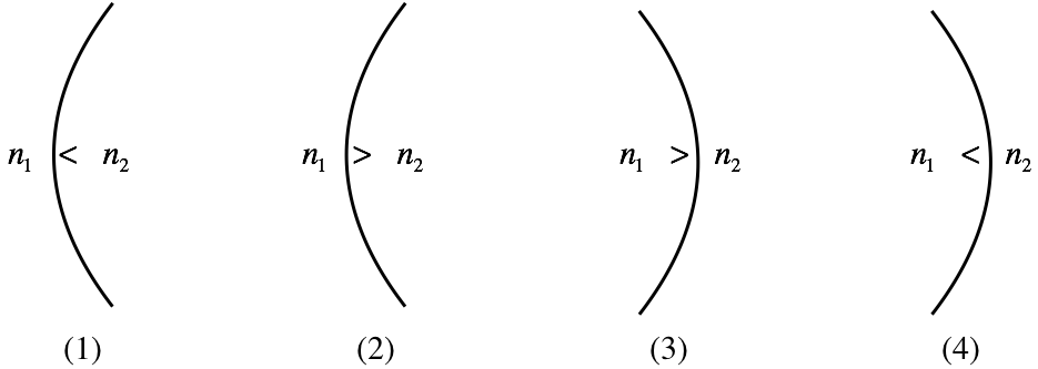
In Section 4.1, when we completed plane reflectors, we moved on to plane refractors, and having done spherical reflections, we now follow the same progression. There were two possibilities for reflectors – concave and convex. While the same two shapes are available for refractors, there are actually four distinct possibilities, since for each of the two shapes, the transition of media can be either from slower medium to faster, or vice-versa. If we assume light is moving left to right in each of the cases, the diagram below lists all four possibilities.

Figure 4.4.1 – Four Varieties of Spherical Refraction

$varieties_of_spherical_refraction.png$

Before diving into finding images for these cases, let's take a moment to get some sense of what happens to a ray that encounters these boundaries in each case. In particular, we will be looking to see if the ray bends toward or away from the optical axis as it crosses the boundary between the two media. Central to this discussion is the law of refraction, the conceptual basis of which is that a light ray entering a slower medium bends toward the perpendicular to the surface, while a ray that enters a faster medium bends away from this perpendicular.

Figure 4.4.2 – Ray Convergence and Divergence for the Four Cases of Spherical Refraction

$four_spherical_refractions.png$

It is important to note that neither the shape of the border, nor change in the speed of the light, determines by itself the convergence or divergence of rays. Only the combination of both of these factors makes this determination.

Object and Image Distances

As with the case of reflectors, it is clear that the image of an object point on the optical axis is also on the optical axis, because a ray along the optical axis will strike the boundary at a right angle and will pass straight through without bending. Our task is therefore to determine how far the image is from the vertex, given the distance of the object from the vertex. In the diagrams that follow, we will maintain the following conventions:

The object is always to the left of the boundary, and the observer to the right, viewing the light after it passes through.
The shaded region is the one with the higher index of refraction. This means the light travels slower there, and the angle on that side of the boundary is always the smaller one.

In each case, we will look at two rays – one that is along the optical axis, and the other that strikes the boundary off-axis. Backtracking the second ray to the optical axis will locate the image point. We will diagram each of the four cases shown in the figure above...

Figure 4.4.3 – Image of a Point on the Optical Axis – Picture (Case 1)

$image_spherical_refractor_1.png$

Before we go on, it is important to note that for this case, we have assumed that the object is not too close to the refracting surface. Imagine what happens if we move it closer: The angle $\theta_1$ grows, which causes angle $\theta_2$ to grow, according to Snell's law. But if $\theta_2$ grows too much, then the outgoing ray may not converge to the axis on its way to the eye. If we move the object close enough to the refracting surface, then the image ends up on the left side of the surface. The light rays don't actually cross the axis there, but the eye sees the light coming from that point.

As with the case of the spherical reflector, we need to make the approximation that the spherical surface is flat. The geometry here is significantly more involved than it was for the reflector, because in the reflection case, the two angles at the surface were equal, while here they are related by Snell's law (Equation 3.6.4). The simplest approach to this geometry is to first reduce the clutter by separating the three right triangles involved and naming all the relevant angles...

Figure 4.4.4a – Image of a Point on the Optical Axis – Geometry (Case 1)

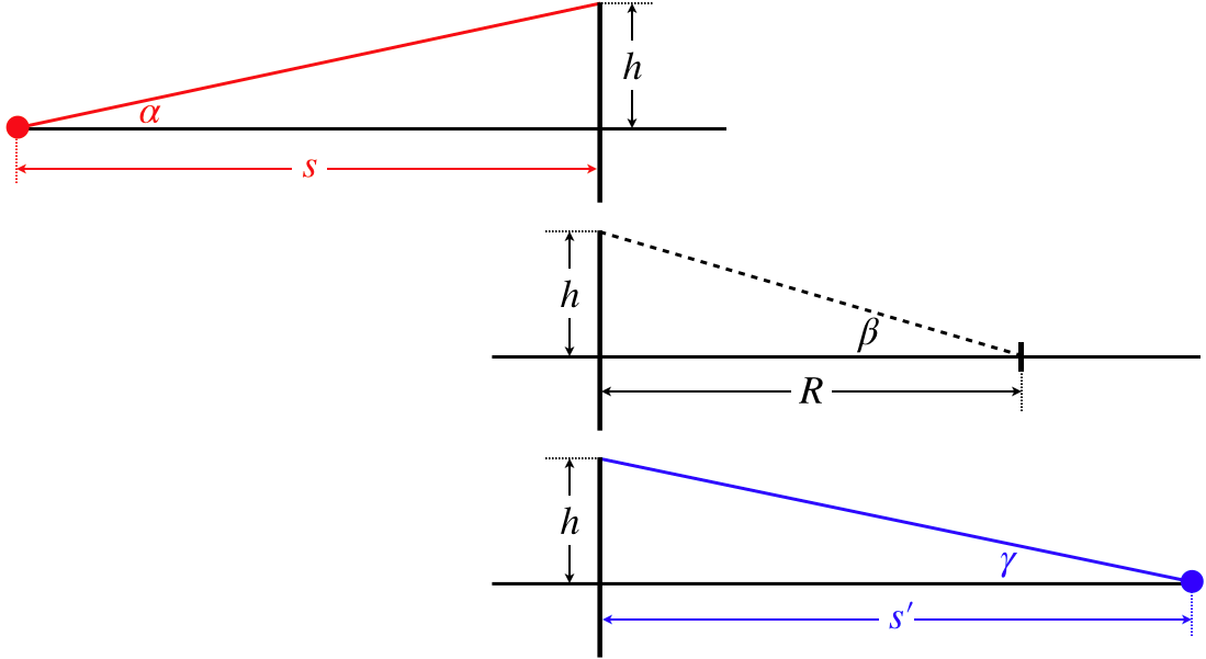
$spherical_refractor_geometry_1.png$

We can now relate these angles to the sides of the triangles, using our usual small-angle approximation:

\[\begin{array}{l} \alpha\approx\tan\alpha = \dfrac{h}{s} \\ \beta\approx\tan\beta = \dfrac{h}{R} \\ \gamma\approx\tan\gamma = \dfrac{h}{s'} \end{array}\]

Though the pictures are different, so far this is actually no different from what we obtained in Equations 4.3.2. The difference comes in how we relate these angles to each other. In the case of the spherical reflector, the law of reflection gave us the simple relation of Equation 4.3.1. Here we have to employ Snell's law to obtain a link between these angles. To see how these angles relate to each other, one more diagram is called for, this one focusing on the point at the boundary where the ray passes through.

Figure 4.4.4b – Image of a Point on the Optical Axis – Geometry (Case 1)

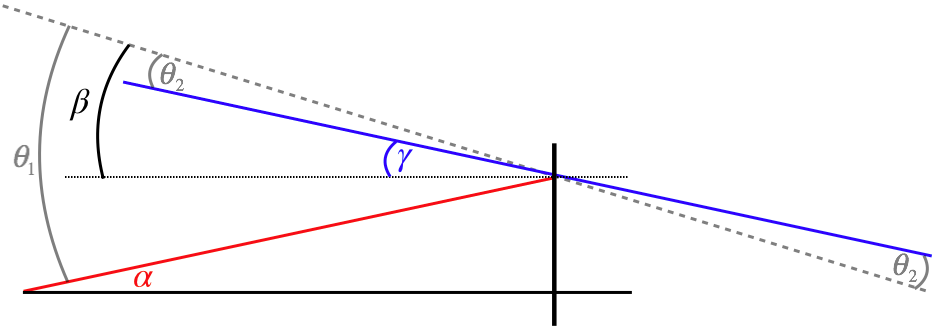
$spherical_refractor_geometry_2.png$

This diagram includes the angles from the three triangles, as well as the two refraction angles, $\theta_1$ and $\theta_2$. We can now do the geometry necessary to relate them to each other, and combine them with the triangle equations above:

\[\theta_1 = \alpha+\beta = \dfrac{h}{s} + \dfrac{h}{R} \;,\;\;\;\;\;\theta_2 = \beta - \gamma = \dfrac{h}{R} - \dfrac{h}{s'}\]

We also have Snell's law relating $\theta_1$ and $\theta_2$, along with the small angle approximation $\sin\theta\approx\theta$:

\[n_1\sin\theta_1 = n_2\sin\theta_2\;\;\;\Rightarrow\;\;\;n_1\theta_1 \approx n_2\theta_2\]

Plugging this in above gives a result reminiscent of Equation 4.3.3, with the difference coming from the two indices of refraction:

\[\left. \begin{array}{l} n_1\theta_1 = n_1\left(\dfrac{h}{s} + \dfrac{h}{R}\right) \\ n_2\theta_2 = n_2\left(\dfrac{h}{R} - \dfrac{h}{s'}\right) \\ n_1\theta_1 = n_2\theta_2 \end{array} \right\} \;\;\; \dfrac{n_1}{s}+\dfrac{n_2}{s'} = \dfrac{n_2-n_1}{R} \]

Although this is different from the result of the reflector, we can still define a focal length. As before, we do this by solving for the image distance of an object at an infinite distance:

\[\dfrac{n_1}{\infty} + \dfrac{n_2}{f} = \dfrac{n_2-n_1}{R} \;\;\;\Rightarrow\;\;\; f = \dfrac{n_2}{n_2-n_1}R\]

Notice that while the focal length of a reflector is shorter than the radius of the mirror, for a refractor it is longer. So Equation 4.4.4 can be written in terms of the focal length as:

\[\dfrac{n_1}{s} + \dfrac{n_2}{s'} = \dfrac{n_2}{f} \]

The ray traces of the other three cases look different from case 1:

Figure 4.4.5 – Image of a Point on the Optical Axis – Picture (Case 2)

$image_spherical_refractor_2.png$

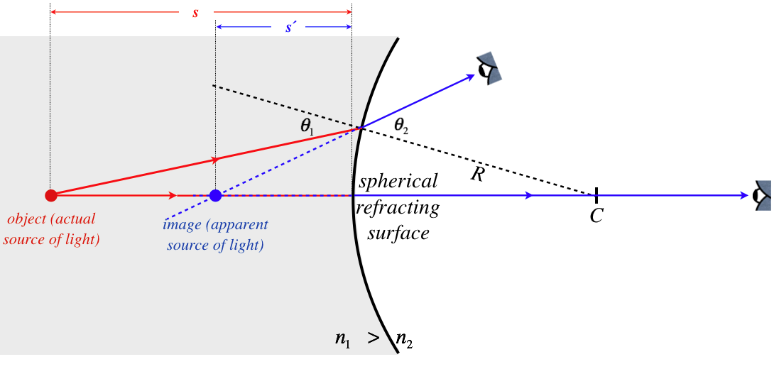
Figure 4.4.6 – Image of a Point on the Optical Axis – Picture (Case 3)

$image_spherical_refractor_3.png$

Figure 4.4.7 – Image of a Point on the Optical Axis – Picture (Case 4)

$image_spherical_refractor_4.png$

We will not re-work the geometry for cases 2 though 4, but rather will state without proof that the same relationship between the object distance, image distance, and radius of curvature holds, provided the sign conventions we have established are maintained.

Checking Sign Conventions

Let's do a quick check to see if the diagrams above match what we expect from the formula and sign conventions.

Case 1:

As we saw with the reflector, whenever a surface causes rays to converge, the image can either be real or virtual, depending upon the object distance. If the object is closer to the surface than the focal point ($s<f$), the image is virtual ($s'<0$), and if it is farther from the surface than the focal point ($s>f$), the image is real ($s'>0$). In Figure 4.4.3, the object distance is greater than the focal length. We know this because the ray shown converges down to the optical axis. If it was at the focal point, the ray would converge to a line parallel to the optical axis, and if it was inside the focal point, it would not even converge as far as the parallel.

The object is on the incoming side of the surface and is farther from the surface than the focal point: $s>0$, $s>f$
The center of the sphere is on the outgoing side: $R>0$
The light is going from faster medium to slower medium: $n_2>n_1$, $f=\dfrac{n_2}{n_2-n_1}R>0$
Rearranging Equation 4.4.6, we can show that the image distance must be positive, which agrees with the diagram that shows the image to be on the outgoing side of the surface:

\[\dfrac{n_2}{s'} = \dfrac{n_2}{f} - \dfrac{n_1}{s}\]

With $s>f>0$ and $n_2>n_1$, the first term on the right hand side of this equation must be greater than the second term, making the difference (and $s'$) positive.

Example $\PageIndex{1}$

Figure 4.4.3 shows the image to be farther from the surface than the center of the sphere. For the conditions given for that diagram, confirm mathematically that this must be true.

Solution

Rearranging Equation 4.4.4, we have:

\[\dfrac{n_1}{s}+\dfrac{n_1}{R} = \dfrac{n_2}{R} - \dfrac{n_2}{s'} \]

The left hand side of this equation is positive, so on the right hand side the second term must be smaller than the first term, which means the second term's denominator must be larger than the first's: $s'>R$.

Case 2:

In this case, the surface causes the rays to diverge, so the nature of the image is not affected by the magnitude of the object distance.

The object is on the incoming side of surface: $s>0$
The center of the sphere is on the outgoing side: $R>0$
The light is going from slower medium to faster medium, which means that the focal length and radius have opposite signs (i.e. the focal point is on the opposite side of the surface as the center point): $n_2<n_1$, $f=\dfrac{n_2}{n_2-n_1}R<0$
Rearranging Equation 4.4.6, we can show that the image distance must be negative, which agrees with the diagram that shows the image to not be on the outgoing side of the surface:

\[\dfrac{n_1}{s} = \dfrac{n_2}{f} - \dfrac{n_2}{s'}\]

The left hand side of this equation is positive, and the first term on the right hand side is negative. This means that $s'$ must be negative.

Example $\PageIndex{2}$

An object is viewed through a spherical refracting surface like that in case 2, with $n_1=1.2$ and $n_2=1.0$. Can the image be seen at a distance from the surface equal to the radius of the sphere? If so, determine the distance that the object must be from the surface (in terms of the radius of the sphere) for this to happen.

Solution

For this case, the $s'<0$ and $R>0$, so the condition we are asked to check is: $s' = -R$. Plugging this into Equation 4.4.4, we have:

\[\dfrac{n_1}{s} + \dfrac{n_2}{-R} = \dfrac{n_2-n_1}{R} \;\;\;\Rightarrow\;\;\; \dfrac{n_1}{s} = \dfrac{2n_2-n_1}{R}\nonumber\]

So we see that this is only a possibility when $2n_2>n_1$, which happens to be the case here. Plugging in the values for $n_1$ and $n_2$, we find that the object must be a distance 1.25 times the radius of the sphere from the surface.

Cases 3 and 4:

The remaining cases follow similarly with the first two. Case 3 involves converging rays ($f>0$) like Case 1, which comes about because $R<0$ (center is not on the outgoing side), and $n_2-n_1<0$ (light going from slower medium to faster one). It should be noted that Case 3, like Case 1, includes a possibility that is not depicted in its associated figure. Figure 4.4.6 assumes that the object point is sufficiently far from the refracting surface (making $\theta_1$ sufficiently large) that Snell's law will result in the ray being bent back down to the axis. The fact that a second figure was not drawn for either Case 1 or Case 3 should not confuse the reader into thinking that having the rays converge back to the axis is the only possibility, or that the mathematical result is any different in such situations (the sign conventions make it all work out!).

Case 4 involves diverging rays ($f<0$) like case 2 because $R<0$ and $n_2-n_1>0$.

Lateral Magnification

We do not need to go through all the principal rays to derive the lateral magnification relation for the spherical refractor. We can simply note that a ray coming from the tip of an object arrow that approaches the refractor parallel to the optical axis is a distance $y$ from the optical axis. Then after hitting the surface, it either converges toward or away from the focal point. The tip of the image arrow then lies on this angled part of the ray, a distance of $\pm y'$ from the axis. These two heights form similar right triangles. The right triangle associated with the object has legs of length $y$ and $f$, while the right triangle associated with the image has legs of length $y'$ and $s'-f$. Setting the ratios of the lengths of their legs equal, we have an expression for the lateral magnification:

\[M = \dfrac{y'}{y} = -\dfrac{s'-f}{f} \]

From Equation 4.4.6, we have:

\[\dfrac{n_1}{s} = n_2\left(\dfrac{1}{f}-\dfrac{1}{s'}\right) \;\;\;\Rightarrow\;\;\; \dfrac{n_1}{n_2s}=\dfrac{s'-f}{fs'} \;\;\;\Rightarrow\;\;\; M=-\dfrac{n_1}{n_2}\dfrac{s'}{s} \]

Comparing this lateral magnification with that of the spherical reflector, we see that a factor of $\frac{n_1}{n_2}$ has been introduced. It seems clear that a greater difference in the two indices of refraction will cause the light to refract more, which should lead to more magnification. Comparing with the result from the plane refractor (Equation 4.1.6), we see that the lateral magnification is confirmed to be +1.