
1.2: Vector Multiplication


- Last updated
- Nov 8, 2022
- Save as PDF

( \newcommand{\kernel}{\mathrm{null}\,}\)
Now we know how to do some math with vectors, and the question arises, “If we can add and subtract vectors, can we also multiply them?” The answer is yes and no. It turns out that there is not one unique way to define a product of two vectors, but instead there are two…
Scalar Product
Soon we will be looking at how we can describe the effect that a force pushing on an object has on its speed as it moves from one position to another. The force is a vector, because it has a magnitude (the amount of the push) and a direction (the way the push is directed). And the movement of the object is also a vector (tail is at the object’s starting point, and head is at its ending point). It will turn out that this effect is describable mathematically as the product of the amount of force and the amount of movement. This is simple to compute if the push is along the direction of movement, but what if it is not? It turns out that only the amount of push that acts in the direction of the movement will affect the object's speed.
We therefore would like to introduce the notion of the projection of one vector onto another. The best description of this is, "the amount of a given vector that points along the other vector." This could be imagined as the “shadow” one vector casts upon another vector:
Figure 1.2.1 – Projecting One Vector Onto Another
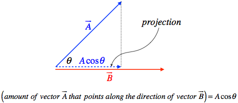
So if we want to multiply the length of a vector by the amount of a second vector that is projected onto it we get:
(projection of →A onto →B)(magnitude of →B)=(Acosθ)(B)=ABcosθ
This is the first of the two types of vector multiplication, and it is called a scalar product, because the result of the product is a scalar. We usually write the product with a dot (giving its alternative name of dot product):
→A⋅→B≡ABcosθ,θ=anglebetween→Aand→B
Example 1.2.1
The vector →A has a magnitude of 120 units, and when projected onto →B, the projected portion has a value of 105 units. Suppose that →B is now projected onto →A, and the projected length is 49 units. Find the magnitude of →B.
- Solution
-
The factor that determines the length of the projection is cosθ. The angle between the two vectors is the same regardless of which vector is projected, so the factor is the same in both directions. The projection of →A onto →B is 7/8 of the magnitude of →A, so the magnitude of →B must be 8/7 of its projection, which is 56 units. Note that when the projection of one vector is multiplied by the magnitude of the other, the same product results regardless of which way the projection occurs. That is, the scalar product is the same in either order (i.e. it is commutative).
Note that a scalar product of a vector with itself is the square of the magnitude of that vector:
→A⋅→A=A2cos0=A2
It should be immediately clear what the scalar products of the unit vectors are. They have unit length, so a scalar product of a unit vector with itself is just 1.
ˆi⋅ˆi=ˆj⋅ˆj=ˆk⋅ˆk=1
They are also mutually orthogonal, so the scalar products with each other are zero:
ˆi⋅ˆj=ˆj⋅ˆk=ˆk⋅ˆi=0
This gives us an alternative way to look at components, which are projections of a vector onto the coordinate axes. Since the unit vectors point along the x, y, and z directions, the components of a vector can be expressed as a dot product. For example:
→A⋅ˆi=(Axˆi+Ayˆj+Azˆk)⋅ˆi=Axˆi⋅ˆi1+Ayˆj⋅ˆi0+Azˆk⋅ˆi0
Unit vectors also show us an easy way to take the scalar product of two vectors whose components we know. Start with two vectors written in component form:
→A=Axˆi+Ayˆj
→B=Bxˆi+Byˆj
then just do "normal algebra," distributing the dot product as you would with normal multiplication:
→A⋅→B=(Axˆi+Ayˆj)⋅(Bxˆi+Byˆj)=(AxBx)ˆi⋅ˆi1+(AyBx)ˆj⋅ˆi0+(AxBy)ˆi⋅ˆj0+(AyBy)ˆj⋅ˆj1=AxBx+AyBy
If we didn’t have this simple result, think about what we would have to do: We would need to calculate the angles each vector makes with (say) the x-axis. Then from those two angles, we need to figure out the angles between the two vectors. Then we would need to compute the magnitudes of the two vectors. Finally, with the magnitudes of the vectors and the angle between the vectors, we could finally plug into our scalar product equation.
Alert
With two different ways to compute a scalar product, it should be clear that the simplest method to use will depend upon what information is provided. If you are given (or can easily ascertain) the magnitudes of the vectors and the angle between them, then use Equation 1.2.2, but if you are given (or can easily ascertain) the components of the vectors, use Equation 1.2.7.
Example 1.2.2
The two vectors given below are perpendicular to each other. Find the unknown z-component.
→A=+5ˆi−4ˆj−ˆk→B=+2ˆi+3ˆj+Bzˆk
- Solution
-
The scalar product of two vectors is proportional to the cosine of the angle between them. This means that if they are orthogonal, the scalar product is zero. The dot product is easy to compute when given the components, so we do so and solve for Bz:
0=→A⋅→B=(+5)(+2)+(−4)(+3) +(−1)(Bz)⇒Bz=−2
The scalar product of two vectors in terms of column vectors works exactly how you would expect – simply multiply the similar components and sum all the products. Or, if you are familiar with matrix multiplication, multiply the transpose (row matrix) of one vector by the column matrix of the other:
→A⋅→B=(AxAyAz)(BxByBz)=AxBx+AyBy+AzBz
Vector Product
As mentioned earlier, there are actually two ways to define products of vectors. If the scalar product involves the amount of one vector that is parallel to the other vector, then it should not be surprising that our other product involves the amount of a vector that is perpendicular to the other vector.
Figure 1.2.2 – Portion of One Vector Perpendicular to Another
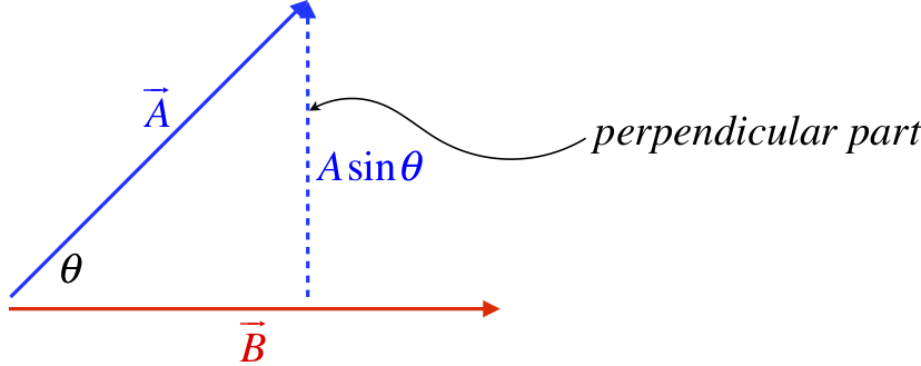
If we take a product like before, multiplying this perpendicular piece by the magnitude of the other vector, we get an expression similar to what we got for the scalar product, this time with a sine function rather than a cosine. For reasons that will be clear soon, this type of product is referred to as a vector product. Because this is distinct from the scalar product, we use a different mathematical notation as well – a cross rather than a dot (giving it an alternative name of cross product). This has a simple (though not entirely useful, at least not in physics) geometric interpretation in terms of the parallelogram defined by the two vectors:
Figure 1.2.3 – Constructing a Vector Product (Magnitude)
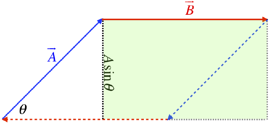
magnitudeof→A×→B=|→A×→B|=|→A||→B|sinθ=ABsinθ
But there is another even bigger difference between the vector and scalar products. While the projection always lands parallel to the second vector, the perpendicular part implies an orientation, since the perpendicular part can point in multiple directions. Any quantity that has an orientation has the potential to be a vector, and in fact we will define a vector that results from this type of product as follows: If we follow the perimeter of the parallelogram above in the direction given by the two vectors, we get a clockwise orientation [Would we get the same orientation if the product was in the opposite order: →B × →A?]. We turn this circulation direction into a vector direction (which points in a specific direction in space) using a convention called the right-hand-rule:
Convention: Right-Hand-Rule
Point the fingers of your right hand in the direction of the first vector in the product, then orient your hand such that those fingers curl naturally into the direction of the second vector in the product. As your fingers curl, your extended thumb points in a direction that is perpendicular to both vectors in the product. This is the direction of the vector that results from the cross product.
If we perform the cross product with the vectors in the opposite order, our fingers curl in the opposite direction, which makes our thumb point in the opposite direction in space. This means that the cross product has an anticommutative property:
→A×→B=−→B×→A
A cross product of any vector with itself gives zero, since the part of the first vector that is perpendicular to the second vector is zero:
|→A×→A|=A2sin0=0
As with the scalar product, the vector product can be easily expressed with components and unit vectors. The vector products of the unit vectors with themselves are zero. Each of the unit vectors is at right angles with the other two unit vectors, so the magnitude of the cross product of two unit vectors is also a unit vector (since the sine of the angle between them is 1).
Convention: Right-handed Coordinate Systems
We will always choose a right-handed coordinate system, which means that using the right-hand-rule on the +x to +y axis yields the +z axis.
In terms of the unit vectors, we therefore have:
ˆi׈i=ˆj׈j=ˆk׈k=0
and
ˆi׈j=−ˆj׈i=ˆk,ˆj׈k=−ˆk׈j=ˆi,ˆk׈i=−ˆi׈k=ˆj
This allows us to do cross products purely mathematically (without resorting to the right-hand-rule) when we know the components, as we did for the scalar product. Again start with two vectors in component form:
→A=Axˆi+Ayˆj
→B=Bxˆi+Byˆj
then, as in the case of the scalar product, just do "normal algebra," distributing the cross product, and applying the unit vector cross products above:
→A×→B=(Axˆi+Ayˆj)×(Bxˆi+Byˆj)=(AxBx)ˆi׈i0+(AyBx)ˆj׈i−ˆk+(AxBy)ˆi׈j+ˆk+(AyBy)ˆj׈j0=(AxBy−AyBx)ˆk
It is not obvious right now how we will use the dot and cross product in physics, but it is coming, so it’s a good idea to get a firm grasp on these important tools now.