
1.3: Straight-Line Motion


- Last updated
- Nov 8, 2022
- Save as PDF

( \newcommand{\kernel}{\mathrm{null}\,}\)
There is nothing more fundamental in the study of physics than motion. We will bring a lot of mathematics to bear on this subject (including the vectors we just learned about), but we are going to start as easy as possible – with motion that remains on a straight line. This simplifies our task in several ways, the primary of which is the reduction of vectors to simple positive and negative quantities (one direction is arbitrarily chosen as the positive direction, and the opposite direction is negative).
Displacement
In order for motion to occur for an object, obviously its position must change from one instant in time to another. We will refer to the coordinate position of the straight line on which the object moves as x(t). A change in this position we call the displacement, and refer to it as a change in position:
displacement=Δx≡xf−xo
Alert
It’s a good idea to get used to this now, as you will use it throughout the Physics 9-series: When referring to a time-dependent quantity, the “delta” (∆) means “after minus before,” or “final minus initial.”
Notice that if the final position is a smaller number than the initial position, then the object has a negative displacement. Eventually we will treat displacement as a vector, but for our straight-line motion, the sign of the value provides all the information we need about the direction. In this text you will receive several warnings about the precise use of physics language, which is frequently at odds with how the same words are used in casual conversation. Here is the first example:
Alert
“Displacement” sounds a lot like “distance covered.” Walking a mile to the store and back again is a two mile walk, but the displacement in this case is not two miles. Displacement is a vector whose magnitude is the distance between the starting and ending points, and whose direction points from the starting point to the ending point.
Average Velocity
Of course, there is more to motion than just displacement. We will generally also be interested in how fast that displacement occurs. We therefore define a rate called the average velocity thus:
average velocity=vave≡ΔxΔt=xf−xotf−to
Since we know displacement is a vector (of course in our current simple 1-dimensional model it can only have two directions), then average velocity must be a vector as well.
Instantaneous Velocity
Just talking about the before and after gets pretty boring, so what do we do about during? That is, how do we define a velocity at a single moment in time – the instantaneous velocity? Well, we know the answer to this from calculus. We start with our idea of average velocity, and just shrink the time span down very small, until it vanishes:
instantaneous velocity=v=limΔt→0ΔxΔt=dxdt
Average and Instantaneous Acceleration
We take our discussion of motion to one level more – we consider that things might speed up or slow down. Just as we defined average velocity in terms of before and after positions, we also define average acceleration in terms of before and after (instantaneous) velocities:
average acceleration=aave=ΔvΔt=vf−votf−to
And, as before, we use calculus to extend this notion of average acceleration to instantaneous acceleration, which we describe as the amount that our object is speeding up or slowing down at a single moment in time:
instantaneous acceleration=a=limΔt→0ΔvΔt=dvdt=d2xdt2
Alert
Another language warning – In standard English parlance, we are used to reserving the word “acceleration” to mean only “speeding up.” In physics it means specifically the rate of change of velocity, which for straight line motion includes both speeding up and slowing down (for multi-dimensional motion it gets even trickier).
Example 1.3.1
If a moving object is slowing down, is it possible that the magnitude of its acceleration is increasing? If an object is speeding up, is it possible that the magnitude of its acceleration is decreasing? In either of these cases, can the magnitude of the acceleration be zero? Explain.
- Solution
-
If an object is slowing down, then it is experiencing an acceleration in the direction opposite to its motion. If this acceleration increases in magnitude, then it slows down faster. So naturally it can be slowing down as the acceleration magnitude increases. Similarly, as an object is speeding up, it is experiencing an acceleration in the direction of its motion. If the magnitude of this acceleration decreases, then the rate at which it speeds up decreases, but it is still speeding up. If the object is either slowing down or speeding up, then its velocity must be changing, and the acceleration cannot be zero.
Motion Diagrams
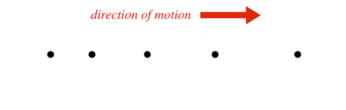
A motion diagram starts as merely a series of collinear dots that represent the position of an object at different equally-spaced intervals of time. You can think of it as a time-lapse photograph using a strobe light. There is one other piece of information that goes with this starting diagram: the direction that the object is moving. An example of this starting point might be this:
Figure 1.3.1a – Creating a Motion Diagram
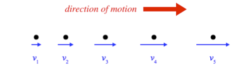
From this we need to somehow extract the instantaneous velocity (magnitude and direction, which may be changing) at each position, and the acceleration (magnitude and direction, assumed to be constant throughout) of the object. At this point we are only working qualitatively, so our goal is to sketch onto the diagram velocity vectors at each dot that have magnitudes and directions that approximately represent the velocities of the object at those points (v1, v2, etc.), keeping in mind that the time intervals between dots are all the same, and the acceleration is constant throughout. You can do this intuitively (it must be going faster if it covers more distance in the same time), or you can figure it out from Equation 1.3.2. Adding the instantaneous velocity vectors to the above diagram makes it look like this:
Figure 1.3.1b – Creating a Motion Diagram
Now for acceleration. Since we are assuming constant acceleration (at least for the five-data-point interval we are considering), the average acceleration equals the instantaneous acceleration. With each dot being separated by the same time interval, the acceleration between dots is proportional to the velocity changes (magnitude and direction), and in this case of constant acceleration, is the same between every pair of dots:
a=constant=aave=ΔvΔt=v2−v1t2−t1=v3−v2t3−t2=...
Putting this into the diagram gives:
Figure 1.3.1c – Creating a Motion Diagram
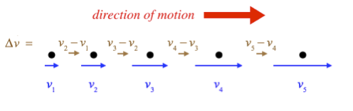
Note that Δv is determined using the usual tail-to-head vector addition, which in one dimension just consists of keeping the signs straight.
If we didn’t know whether or not the acceleration was constant, we could make a good guess by comparing the Δv’s. Notice that we need two dots to determine the average velocity for a single time interval, since two dots gives us a displacement. But if we want to know how the speed is changing (i.e. the acceleration), we need three dots. If dots #1 and #2 are closer together than dots #2 and #3, we know the object has sped up, and if the first two dots are father apart, then the object is slowing down. So when we label our motion diagram, we can arbitrarily draw-in the first velocity vector on the first dot, but we can’t add the velocity vector to the second dot if there is no third dot present to show us if the object is object is going faster, slower, or the same speed at the second dot. The more changes we want to consider (like if we want to know about a changing acceleration), the more dots we need.
This is in fact the nature of calculus – the change of a change of a change, etc, requires an additional measurement of position for each additional change computed. So the motion diagram only needs three dots if the acceleration is known (or assumed) to be constant, but to confirm that it is constant requires four dots.