3.1: The Work - Energy Theorem

Ignoring Directional Changes

For a large number of applications in mechanics, we are not interested in how a force causes the direction of motion of an object to change. In these cases, we only care about how that force changes the speed of the object. By now we know how much of a pain vectors can be, so having an alternative to Newton’s second law to solve problems where only changes in speed are of interest is a welcome improvement. To see how we get to such a place, we need to go back to what we previously said about acceleration, and how it breaks into perpendicular parts – one that is parallel to the velocity (the “speeding-up/slowing-down” part), and the part that is perpendicular to the velocity (the “changing direction” part). We expressed this mathematically in Equation 1.6.12. We will now restrict our attention to the first term. Note that restricting ourselves to the part of the acceleration parallel to the direction of motion means we also restrict ourselves only to the component of the net force parallel to the motion.

Kinetic Energy and the Work-Energy Theorem

We have a neat trick that allows us to relate the change of the speed to the net force. The net force is proportional to the time derivative of the velocity vector, and we can use the product rule for derivatives of dot products of vectors, so let's take a derivative of the square of the velocity:

\[ \dfrac{d}{dt}v^2 = \dfrac{d}{dt} \left( \overrightarrow v \cdot \overrightarrow v \right) = \dfrac{d \overrightarrow v}{dt} \cdot \overrightarrow v + \overrightarrow v \cdot \dfrac{d \overrightarrow v}{dt} = 2 \overrightarrow a \cdot \overrightarrow v \]

To get to the net force, we multiply both sides by the mass of the object and divide both sides by 2:

\[ \dfrac{d}{dt} \left( \frac{1}{2}m v^2 \right) = \left( m \overrightarrow a \right) \cdot \overrightarrow v = \overrightarrow F_{net} \cdot \overrightarrow v \]

This makes some sense. The rate of change on the left side of this equation only depends upon the rate at which the speed changes (it is insensitive to changes in direction), and the dot product on the right side ensures that only the projection of the net force along the direction of motion (i.e. the direction of the velocity) plays a role. The part of the net force that causes the object to change direction is thrown away. We can take this a little bit further by expressing the velocity vector on the right side as a tiny displacement (which we will call \(\overrightarrow {dl}\)) divided by the tiny time interval. Multiplying both sides by \(dt\) then gives an equation that expresses a small change in the quantity \(\frac{1}{2}mv^2\) (called the kinetic energy) due to a net force acting on the object as it displaces a small amount \(\overrightarrow {dl}\).

\[ \dfrac{d}{dt} \left( \frac{1}{2}m v^2 \right) = \overrightarrow F_{net} \cdot \dfrac{\overrightarrow {dl}}{dt} \;\;\; \Rightarrow \;\;\; d\left( \frac{1}{2}m v^2 \right) = \overrightarrow F_{net} \cdot \overrightarrow {dl} \]

Suppose the object now undergoes several displacements, so that the change in the kinetic energy is no longer infinitesimal. This is tricky business, as each displacement may be the same (if it moves in a straight line), or it may change direction (if it follows a curvy path). Also, the net force on the object might change as the object moves from one place to another. We express the sum of many infinitesimals as an integral, and since the sum of the right side of this equation depends upon the directions of many displacements, this particular type of integral is called a line integral. This does not mean that the displacements are along a straight line, however – here the word "line" is rather misleading – the word "trajectory" might be better.

Of course, the left side of this equation is simply a small number, and adding those up does not depend upon anything as complicated as a trajectory, so it ends up being just a change from the beginning of the path to the end. If we call the start of the journey \(A\) and the end \(B\), then we can express the totals for the whole journey as:

\[ \Delta \left( \frac{1}{2} mv^2 \right) = \frac{1}{2} mv_B^2 - \frac{1}{2} mv_A^2 = \int \limits_A^B \overrightarrow F_{net} \cdot \overrightarrow {dl} \]

The line integral on the right side of this equation is called the work done (by the net force) going from the initial to final positions. We can (and later, will) discuss the work done by individual forces, and the work done by the net force is the total of all of those works. We will often write the above equation with the following abbreviated notation:

\[ \Delta KE = W_{tot} \left(A \rightarrow B \right) \]

In words, this reads: "The change of an object's kinetic energy when it changes its position from \(A\) to \(B\) equals the work done on it by all forces on it, computed over a well-defined path connecting those endpoints." This is known as the work-energy theorem. It does exactly what we set out to do – it expresses the effect forces have on the change in an object's speed, with no regard to its directional changes. It doesn't solve any problem that can't be solved by Newton's second law, and in fact for some cases it isn't even any easier to work with. But for other cases is it much easier to work with, as we will see, and these are the cases for which this approach was invented.

These new quantities of kinetic energy and work have units of what we will more generically refer to as energy, and we give energy units their own name:

\( \left[ KE \right] = \dfrac{kg \cdot m^2}{s^2} = \;"Joules"\;\;(J) \)

Example \(\PageIndex{1}\)

A single force which varies in magnitude and direction in space acts upon an object, and is given by the equation below. Find the change in the object's kinetic energy as it moves from the origin along the \(+x\)-axis a distance of 2m.

\[ \overrightarrow F \left(x,y \right) = \left( \alpha x^2 + \beta y^3 \right) \widehat i + \left( \beta x^3 + \alpha y^2 \right) \widehat j , \;\;\;where: \;\; \alpha = 2.4 \frac{J}{m^2} \;\; and \;\; \beta = 4.5 \frac{J}{m^3} \nonumber \]

Solution

This is a direct application of the work-energy theorem, which means it consists entirely of computing a line integral. To do this, we first need to define the path mathematically, and all of the tiny displacements \(\overrightarrow {dl} \) along that path. The path in this case is pretty simple – it is a straight line along the \(x\)-axis from the origin (\(0m,0m\)) to the point (\(2m,0m\)). Along this path, the value of \(y\) remains a constant zero. The direction of every infinitesimal displacement is the \(+\widehat i \) direction, and the magnitude of each displacement is simply \(dx\). The work integral therefore becomes:

\[ W \left(A \rightarrow B \right) = \int \limits_A^B \overrightarrow F \cdot \overrightarrow {dl} = \int \limits_{x=0m}^{x=2m} \overrightarrow F \cdot \left( dx\; \widehat i \right) \nonumber \]

Now we just need to plug in for the force. The force must be evaluated at each point on the path, and since the value of \(y\) is zero on the entire path, we can set \(y=0\) in the force vector, simplifying things greatly:

\[ \overrightarrow F \left(on\;the\;path\right) = \left( \alpha x^2 \right) \widehat i + \left( \beta x^3 \right) \widehat j \nonumber \]

The dot product of this vector with the tiny displacement vector simplifies things even more:

\[ \overrightarrow F\left(on\;the\;path\right) \cdot \overrightarrow {dl} = \left[\left( \alpha x^2 \right) \widehat i + \left( \beta x^3 \right) \widehat j \right] \cdot \left[ dx\; \widehat i \right] = \alpha x^2dx \nonumber\]

Finally, we just perform the integral and apply the work-energy theorem:

\[ \Delta KE = \int \limits_{0m}^{2m} \alpha x^2 dx = \left[ \frac{1}{3} \alpha x^3 \right]_{0m}^{2m} = \boxed{6.4J} \nonumber \]

Line Integrals

As you can tell from the example above, the hardest part of using the work-energy theorem is setting up the line integral. There are several elements that need to be kept in mind:

1. define a direction for the tiny displacement vectors for every point on the path

The direction of the tiny displacement vectors (which we will assume to be in the (\(x,y\)) plane will have components equal to the displacements in the \(x\) and \(y\) directions:

\[ \overrightarrow {dl} = dx \; \widehat i + dy \; \widehat j \]

2. write the magnitude of the tiny displacements in terms of the integration variable

The displacement vector as written above doesn't tell us much. We also need to include the path for this to be useful. Since we are assuming that everything is in the (\(x,y\)) plane, the path can be expressed as a relationship between the variables \(x\) and \(y\). For example, if the path is a straight line, then we can write \(y=mx+b\). In this case, we can replace the \(dy\) in the displacement vector:

\[ \dfrac{dy}{dx}=m \;\;\; \Rightarrow \;\;\; dy = m\;dx \;\;\; \Rightarrow \;\;\; \overrightarrow {dl} = \left[ \widehat i + m \widehat j \right] dx \]

This puts the displacement vector in terms of a single variable (\(x\)) for integration (we could of course have instead chosen our integration variable to be \(y\)). More generally, the path could be a function: \(y = f\left( x \right) \), in which case the \(m\) above would be replaced by the derivative of the function. Note also that the path may not even be a function, since it could have multiple \(y\) values for each \(x\) value. [Suffice to say that path integrals have a lot more going on than we will cover in this course, and we'll leave coverage of the more nuanced details to a course in vector calculus.]

3. evaluate the force vector at each point in the path

The force vector will be in terms of \(x\) and \(y\) (i.e. it is defined at all points in space), but in the integral only its value along the path matters, so we can substitute the equation that defines the path (such as \(y=mx+b\) in the case of a straight-line) into the force vector so that it is a function of only one variable, allowing us to do the integral.

4. take the dot product

We of course know how to do this by now, but it is important to remember that it must be done. This step goes back to the start of our discussion of this method. This dot product assures that we are only using the part of the force vector that lies along the tiny displacement, which means we are only using the part of the force vector that changes the speed of the object.

Of course, much more complicated paths than straight lines are possible. The following example illustrates how this is handled.

Example \(\PageIndex{2}\)

Compute the work done on an object by the force given below, along a parabolic path \(y=\lambda x^2\) connecting the origin to the point on the path with an \(x\) value of 1m, where \(\lambda = 0.4m^{-1}\).

\[ \overrightarrow F \left(x,y \right) = \alpha x^2 \; \widehat i + \beta y \; \widehat j , \;\;\; where: \;\; \alpha = 1.5 \frac{J}{m^2} \;\; and \;\; \beta = 3.0 \frac{J}{m} \nonumber \]

Solution

Start by determining the displacement vector as a function of \(x\) along the path:

\[ \left. \begin{array}{l} \overrightarrow {dl} = dx \; \widehat i + dy \; \widehat j \\ y=\lambda x^2 \;\;\; \Rightarrow \;\;\; \dfrac{dy}{dx}=2 \lambda x \;\;\; \Rightarrow \;\;\; dy = 2 \lambda xdx \end{array} \right\} \; \Rightarrow \; \overrightarrow {dl} = \left( \widehat i + 2 \lambda x \; \widehat j \right)dx \nonumber\]

Next write the force vector along the path only (in terms of \(x\)):

\[ \left. \begin{array}{l} \overrightarrow F \left(x,y \right) = \alpha x^2 \; \widehat i + \beta y \; \widehat j \\ y=\lambda x^2 \end{array} \right\} \;\;\; \Rightarrow \;\;\; \overrightarrow F_{on\;path} \left(x \right) = \alpha x^2 \; \widehat i + \beta \lambda x^2 \; \widehat j \nonumber \]

Now for the dot product:

\[\overrightarrow F_{on\;path} \cdot \overrightarrow {dl} = \left[ \left( \alpha x^2\right) \left(1 \right) + \left( \beta \lambda x^2\right) \left( 2 \lambda x \right) \right]dx = \left( \alpha x^2 +2 \beta \lambda^2 x^3 \right)dx \nonumber \]

And finally integrate between the two endpoints, defined in terms of the \(x\) variable that we have put everything in terms of:

\[ W \left(A \rightarrow B \right) = \int \limits_{x=0m}^{x=1m} \left( \alpha x^2 +2 \beta \lambda^2 x^3 \right)dx = \left[ \frac{1}{3}\alpha x^3 +\frac{1}{2} \beta \lambda^2 x^4 \right]_{x=0m}^{x=1m} = \boxed{0.74J} \nonumber \]

Lost Information

It is important to note that while the introduction of the work-energy theorem will simplify things for us with a subset of problems, we do sacrifice some information. By throwing out the part of the force that acts to change the direction of the object, we cannot use this method to determine which way the object is moving after the force acts on it – we only know how fast it is going. Also, we lose information about the time element of the motion between the starting and ending points. This should not be surprising – just because we know how fast something is moving, if we don’t know the directions it takes to get from start to finish, we still don’t know anything about the elapsed time. For example, a projectile thrown into the air will reach the same speed at two different points of time – once on the way up and once on the way down. If we don't know anything about the direction of motion, we don't know which time we are looking at.

To see this another way, consider a situation we are very familiar with – an object moving in a straight line, accelerating at a constant rate. We know that we can write its acceleration in terms of the starting and final velocities using Equation 1.4.3:

\[ 2a\Delta x = {v_f}^2 - {v_o}^2 \]

By Newton’s second law, the acceleration here must have been caused by a (net) force in the same direction, so substituting the ratio of force/mass for the acceleration gives:

\[ 2 \dfrac{F_{net}}{m} \Delta x = {v_f}^2 - {v_o}^2 \;\;\; \Rightarrow \;\;\; F_{net}\Delta x = \frac{1}{2}m{v_f}^2 - \frac{1}{2}m{v_o}^2 \]

This is once again the work-energy theorem (in one dimension, for a constant net force), and we see that it came directly from the kinematics equation from which the time variable had been eliminated.

Work Contributions of Individual Forces

It probably isn’t immediately clear what is to be gained from this work-energy approach. After all, one still has to determine the net force at each point in the path of the object’s motion, so our attempt to escape the tyranny of vectors would appear to be a failure. But there is much more to this story. It begins with the recognition that total work done can be broken into a sum of works done by individual forces:

\[ \begin{array}{l} W_{tot} \left( A \rightarrow B \right) && = && \int \limits_A^B \overrightarrow F_{net} \cdot \overrightarrow {dl} \\ && = && \int \limits_A^B \left( \overrightarrow F_1 + \overrightarrow F_2 + \dots \right) \cdot \overrightarrow {dl}\\ && = && \int \limits_A^B \overrightarrow F_1 \cdot \overrightarrow {dl} + \int \limits_A^B \overrightarrow F_2 \cdot \overrightarrow {dl} + \dots \\ && = && W_1 \left( A \rightarrow B \right) + W_2 \left( A \rightarrow B \right) + \dots \end{array}\]

There are a number of advantages to this, but the one we can see immediately is that if one of the individual forces happens to be everywhere perpendicular to the path of the object from A to B, then the work it contributes is zero, and we can simply ignore it – no need to do the vector addition to add it to the other forces. Consider the following example of pushing a block across a rough horizontal surface. Figure 3.1.1 shows a diagram of what is happening and a FBD of the block.

Figure 3.1.1 – Pushing Block Across a Rough Horizontal Surface

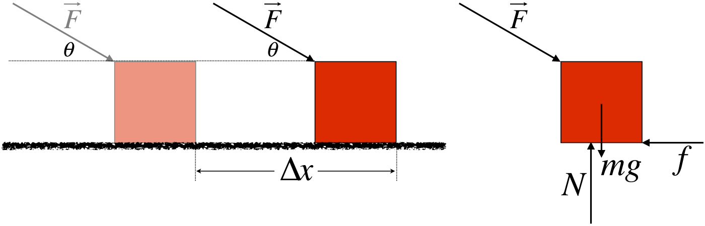
The work done by the net force can be broken down into a sum of the works done by each individual force:

\[ \begin{align} W_{applied\;force} &= \int \limits_A^B \overrightarrow F \cdot \overrightarrow {dl} = F \Delta x \cos \theta \\[5pt] W_{friction} &= \int \limits_A^B \overrightarrow f \cdot \overrightarrow {dl} = f \Delta x \cos180^o = -f \Delta x \\[5pt] W_{gravity} &= \int \limits_A^B \left( -mg \; \widehat j \right) \cdot \overrightarrow {dl} = mg \Delta x \cos90^o = 0 \\[5pt] W_{normal} &= \int \limits_A^B \left( N \; \widehat j \right) \cdot \overrightarrow {dl} = N \Delta x \cos90^o = 0 \\[5pt] W_{tot} &= W_{applied\;force} + W_{friction} + W_{gravity} + W_{normal} = \left(F \cos \theta - f \right) \Delta x =F_{net} \Delta x \end{align} \]

Just by looking at the physical situation it is clear that the gravity and contact forces will play no role in the total work done, as they are always perpendicular to the motion. This greatly reduces the number of forces (and vector addition) we would otherwise have to deal with. Let’s look at some even more compelling examples:

Figure 3.1.2 – Loop-de-Loop

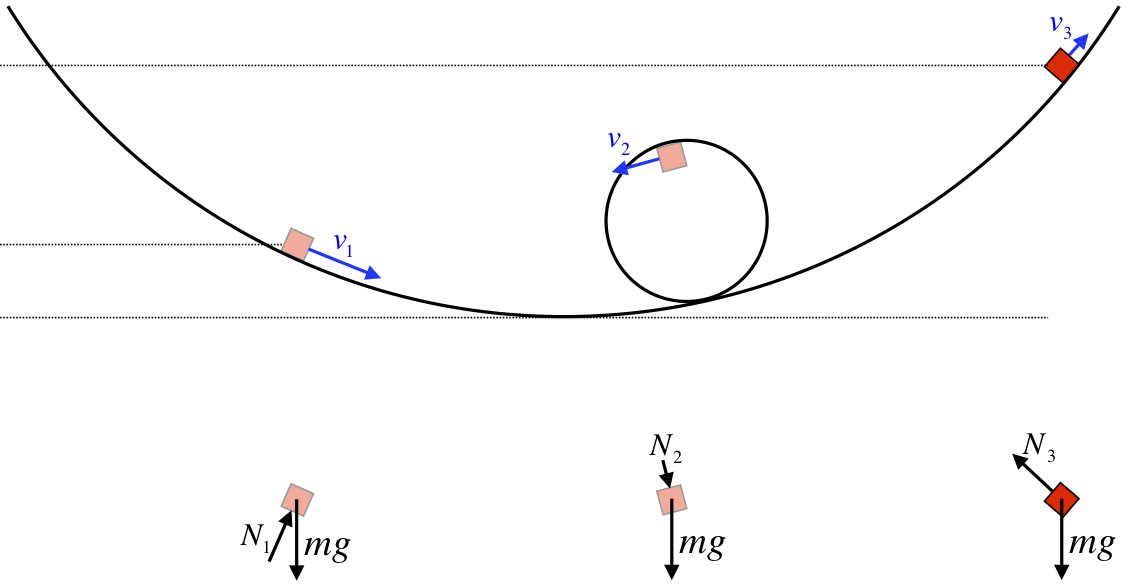
For a block sliding around a frictionless loop-de-loop track, the path it follows is quite complicated. The FBD of the block as it travels along the track includes only two forces – gravity and the normal force by the track. The motion of the block is parallel to the track everywhere, which means it is perpendicular to the normal force everywhere. That means that no matter what our starting and ending points are, the normal force does no work on the block! Of the two forces involved, the normal force is by far the hardest to deal with, since its direction and magnitude change everywhere on the track. but if we are only interested in the speed of the block, we only need to worry about the work done by the gravity force, which has a constant direction and magnitude. We'll come back to the simple result that comes from this shortly.

Figure 3.1.3 – Simple Pendulum

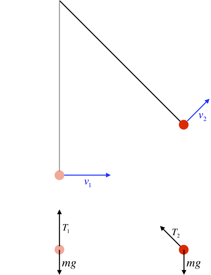
For the simple pendulum, we see the same result for the tension as we found for the normal force in the loop-de-loop example. The tension force remains at right angles to the motion of the bob at the end of the string, so there is no work done by the tension force. If all we care about is the speed of the bob, then we only need to compute the work done by gravity.