
3.4: Energy Conservation Models
- Page ID
- 18395

\( \newcommand{\vecs}[1]{\overset { \scriptstyle \rightharpoonup} {\mathbf{#1}} } \)
\( \newcommand{\vecd}[1]{\overset{-\!-\!\rightharpoonup}{\vphantom{a}\smash {#1}}} \)
\( \newcommand{\id}{\mathrm{id}}\) \( \newcommand{\Span}{\mathrm{span}}\)
( \newcommand{\kernel}{\mathrm{null}\,}\) \( \newcommand{\range}{\mathrm{range}\,}\)
\( \newcommand{\RealPart}{\mathrm{Re}}\) \( \newcommand{\ImaginaryPart}{\mathrm{Im}}\)
\( \newcommand{\Argument}{\mathrm{Arg}}\) \( \newcommand{\norm}[1]{\| #1 \|}\)
\( \newcommand{\inner}[2]{\langle #1, #2 \rangle}\)
\( \newcommand{\Span}{\mathrm{span}}\)
\( \newcommand{\id}{\mathrm{id}}\)
\( \newcommand{\Span}{\mathrm{span}}\)
\( \newcommand{\kernel}{\mathrm{null}\,}\)
\( \newcommand{\range}{\mathrm{range}\,}\)
\( \newcommand{\RealPart}{\mathrm{Re}}\)
\( \newcommand{\ImaginaryPart}{\mathrm{Im}}\)
\( \newcommand{\Argument}{\mathrm{Arg}}\)
\( \newcommand{\norm}[1]{\| #1 \|}\)
\( \newcommand{\inner}[2]{\langle #1, #2 \rangle}\)
\( \newcommand{\Span}{\mathrm{span}}\) \( \newcommand{\AA}{\unicode[.8,0]{x212B}}\)
\( \newcommand{\vectorA}[1]{\vec{#1}} % arrow\)
\( \newcommand{\vectorAt}[1]{\vec{\text{#1}}} % arrow\)
\( \newcommand{\vectorB}[1]{\overset { \scriptstyle \rightharpoonup} {\mathbf{#1}} } \)
\( \newcommand{\vectorC}[1]{\textbf{#1}} \)
\( \newcommand{\vectorD}[1]{\overrightarrow{#1}} \)
\( \newcommand{\vectorDt}[1]{\overrightarrow{\text{#1}}} \)
\( \newcommand{\vectE}[1]{\overset{-\!-\!\rightharpoonup}{\vphantom{a}\smash{\mathbf {#1}}}} \)
\( \newcommand{\vecs}[1]{\overset { \scriptstyle \rightharpoonup} {\mathbf{#1}} } \)
\( \newcommand{\vecd}[1]{\overset{-\!-\!\rightharpoonup}{\vphantom{a}\smash {#1}}} \)
\(\newcommand{\avec}{\mathbf a}\) \(\newcommand{\bvec}{\mathbf b}\) \(\newcommand{\cvec}{\mathbf c}\) \(\newcommand{\dvec}{\mathbf d}\) \(\newcommand{\dtil}{\widetilde{\mathbf d}}\) \(\newcommand{\evec}{\mathbf e}\) \(\newcommand{\fvec}{\mathbf f}\) \(\newcommand{\nvec}{\mathbf n}\) \(\newcommand{\pvec}{\mathbf p}\) \(\newcommand{\qvec}{\mathbf q}\) \(\newcommand{\svec}{\mathbf s}\) \(\newcommand{\tvec}{\mathbf t}\) \(\newcommand{\uvec}{\mathbf u}\) \(\newcommand{\vvec}{\mathbf v}\) \(\newcommand{\wvec}{\mathbf w}\) \(\newcommand{\xvec}{\mathbf x}\) \(\newcommand{\yvec}{\mathbf y}\) \(\newcommand{\zvec}{\mathbf z}\) \(\newcommand{\rvec}{\mathbf r}\) \(\newcommand{\mvec}{\mathbf m}\) \(\newcommand{\zerovec}{\mathbf 0}\) \(\newcommand{\onevec}{\mathbf 1}\) \(\newcommand{\real}{\mathbb R}\) \(\newcommand{\twovec}[2]{\left[\begin{array}{r}#1 \\ #2 \end{array}\right]}\) \(\newcommand{\ctwovec}[2]{\left[\begin{array}{c}#1 \\ #2 \end{array}\right]}\) \(\newcommand{\threevec}[3]{\left[\begin{array}{r}#1 \\ #2 \\ #3 \end{array}\right]}\) \(\newcommand{\cthreevec}[3]{\left[\begin{array}{c}#1 \\ #2 \\ #3 \end{array}\right]}\) \(\newcommand{\fourvec}[4]{\left[\begin{array}{r}#1 \\ #2 \\ #3 \\ #4 \end{array}\right]}\) \(\newcommand{\cfourvec}[4]{\left[\begin{array}{c}#1 \\ #2 \\ #3 \\ #4 \end{array}\right]}\) \(\newcommand{\fivevec}[5]{\left[\begin{array}{r}#1 \\ #2 \\ #3 \\ #4 \\ #5 \\ \end{array}\right]}\) \(\newcommand{\cfivevec}[5]{\left[\begin{array}{c}#1 \\ #2 \\ #3 \\ #4 \\ #5 \\ \end{array}\right]}\) \(\newcommand{\mattwo}[4]{\left[\begin{array}{rr}#1 \amp #2 \\ #3 \amp #4 \\ \end{array}\right]}\) \(\newcommand{\laspan}[1]{\text{Span}\{#1\}}\) \(\newcommand{\bcal}{\cal B}\) \(\newcommand{\ccal}{\cal C}\) \(\newcommand{\scal}{\cal S}\) \(\newcommand{\wcal}{\cal W}\) \(\newcommand{\ecal}{\cal E}\) \(\newcommand{\coords}[2]{\left\{#1\right\}_{#2}}\) \(\newcommand{\gray}[1]{\color{gray}{#1}}\) \(\newcommand{\lgray}[1]{\color{lightgray}{#1}}\) \(\newcommand{\rank}{\operatorname{rank}}\) \(\newcommand{\row}{\text{Row}}\) \(\newcommand{\col}{\text{Col}}\) \(\renewcommand{\row}{\text{Row}}\) \(\newcommand{\nul}{\text{Nul}}\) \(\newcommand{\var}{\text{Var}}\) \(\newcommand{\corr}{\text{corr}}\) \(\newcommand{\len}[1]{\left|#1\right|}\) \(\newcommand{\bbar}{\overline{\bvec}}\) \(\newcommand{\bhat}{\widehat{\bvec}}\) \(\newcommand{\bperp}{\bvec^\perp}\) \(\newcommand{\xhat}{\widehat{\xvec}}\) \(\newcommand{\vhat}{\widehat{\vvec}}\) \(\newcommand{\uhat}{\widehat{\uvec}}\) \(\newcommand{\what}{\widehat{\wvec}}\) \(\newcommand{\Sighat}{\widehat{\Sigma}}\) \(\newcommand{\lt}{<}\) \(\newcommand{\gt}{>}\) \(\newcommand{\amp}{&}\) \(\definecolor{fillinmathshade}{gray}{0.9}\)Systems
Now that we are talking about work done by individual forces, we should make some mention of Newton’s third law. Every individual force is an interaction with two equal-and-opposite forces involved, so how do we know which one of these to use when computing the work done on an object? The work done on an object is calculated using the force on it and the displacement of that same object. So when one drops an apple to earth, the gravity force on the apple multiplied by the distance it drops is the work done on the apple by the gravity force. There is also work done on the earth, as it experiences an equal-and-opposite force, but it displaces much less, so the work done on the earth is much less. So while we can use work as a sort of proxy for force, it is not the same as force - there is not a “Newton's third law” for work.
One thing that will help us keep things straight going forward is the notion of a system. A system is a collection of one or more objects that we have arbitrarily lumped together for accounting purposes. This grouping is isolated from other objects (much like an object in a force diagram), so that forces on it can be taken into account (while other distracting forces can be ignored). With this distinction made, we can also distinguish the work done on a single object as work that is coming from within the system (which may contain other objects) and work that is coming from outside. Breaking the work done into those two types gives a work-energy theorem that looks like this:
\[ W_{tot} = \left( W_1 + W_2 + \dots \right)_{outside} + \left( W_1 + W_2 + \dots \right)_{inside} = \Delta KE \]
For reasons we will see soon, we’ll rearrange terms in such a way that the work done by forces between objects within the system is on the same side of the equation as the change of kinetic energy:
\[ \left( W_1 + W_2 + \dots \right)_{outside} = \Delta KE - \left( W_1 + W_2 + \dots \right)_{inside} \]
This might seem a bit abstract, so let’s return to our example of a block pushed along a rough horizontal surface (Figure 3.1.1). Suppose we make the surface + block a single system. Then how is this equation arranged? The applied force comes from outside the system, and actually so does the gravity force, since we did not include the earth as part of the system. The work done by those forces appear on the left-hand side of the equation. The contact and normal forces are between the block and the table, which are both within the system, so the work done by those forces come from inside the system and appear on the right-hand side (with a minus sign).
Alert
In the future, unless stated otherwise, we will assume that the earth is within the system, so that the work done by gravity always appears on the right-hand side. Note that the work done by gravity on the earth will always be negligible, as the earth’s displacement due to a gravitational interaction with a terrestrial object is vanishingly small.
This may all seem like pointless rearranging, but stay tuned – it will help a great deal with the accounting later.
Total, Mechanical, Potential, and Thermal Energy
So far we have been dancing around the word “energy.” We have only briefly mentioned kinetic energy, in the context of the work-energy theorem, but the very existence of such a term implies the existence of another form of energy. Indeed we do define other forms of energy. We do this in terms of the work done by forces between objects within the system. The summary of this model is:
- The work done on a system by forces that come from outside the system changes the energy contained in that system.
- There are three different types of energy changes that can occur within a system:
- kinetic energy, from the motions of the object(s) within the system
- changes from work done within the system by conservative forces
- changes from work done within the system by non-conservative forces
So far this is just fancy bookkeeping, but next we’ll see how it all comes together. Recall that conservative forces result in work contributions that depend only upon the starting and ending positions of the object moved while under the influence of that force. We therefore define potential energy as a quantity of energy that a system possesses due to the position(s) of the object(s), and the change of that value is (the negative of) the work done by the conservative force:
\[ \Delta PE = PE_B - PE_A = - W \left( A \rightarrow B \right) \]
There are many forms of potential energy – indeed there is a form of PE for every conservative force. Notice that we cannot define a potential energy for a non-conservative force, because PE is defined at specific points in space, so the difference in PE for two points in space is always the same. But for a non-conservative force, different paths between the same two points result in different amounts of work. Incorporating potential energy into our model changes Equation 3.4.3 into:
\[ W_{ext} = \Delta KE + \Delta PE_1 + \Delta PE_2 + \dots - \left( W_1 + W_2 + \dots \right)_{non-conservative} \]
The work done by non-conservative forces between objects within the system is also accounted-for by a change in a quantity of energy, but this quantity does not depend upon the starting and ending positions of objects. Despite this difference with the case of potential energy, we can still write the energy removed from mechanical energy due to non-conservative forces as an increase of energy of a different form – thermal energy. This converts our energy formula into one that contains only changes of forms of energy on the right-hand-side:
\[ W_{ext} = \Delta KE + \Delta PE_1 + \Delta PE_2 + \dots + \Delta E_{thermal} \]
This framework gives us a totally new picture for thinking about energy, if we just choose our system to be “everything.” Then the work done by forces from outside the system is zero (there are no objects to interact with our system from outside!), and the work-energy theorem morphs into:
\[ 0 = \Delta KE + \Delta PE_1 + \Delta PE_2 + \dots + \Delta E_{thermal} \]
When it comes to using this formula, there are few things to note:
- We know \(\Delta KE\) if we know the mass and the beginning and ending speeds of the object.
- We know \(\Delta PE\) if we know the type of conservative force and the beginning and ending positions of the object. (We will soon see how we do this.)
- We know \(\Delta E_{thermal}\) if we know the specific non-conservative force acting, and the path the object takes. However, it is commonly the case that the details of these forces are not provided, in which case either the thermal energy change is given directly, or it is calculated from the above equation.
You may be getting tired of all the renaming of quantities, but there is one more that is helpful for talking about energy. Kinetic and potential energy share the property that they can be converted back-and-forth freely, but thermal energy is a one-way ticket. Once energy is converted to thermal, it doesn’t return to kinetic or potential – we don’t see objects suddenly cool off and start moving. Accordingly, we give the description mechanical energy to the sum of kinetic and potential energy, to distinguish them from thermal energy:
\[0 = \underbrace{\Delta KE + \Delta PE_1 + \Delta PE_2 + \dots}_{\Delta ME} + \Delta E_{thermal} \]
What we have expressed here is known as a conservation principle. In physics, for a quantity to be “conserved” means that its quantity remains fixed over time, and is usually expressed as "\(\Delta something = 0\)." What is particularly interesting here is that the energy changes form or is reallocated into different groupings, but the total remains unchanged. The interpretation of the above equation is that the total energy of a system with no work done on it by forces acting from outside (sometimes referred to as a closed system) is conserved, i.e. the change in its total energy is zero. While all we have done is to rename quantities we have already discussed, this process leads to some useful sub-models for energy conservation that we can use to solve certain characteristic problems. The table below shows the various models we will use.
Figure 3.4.1 – Summary of Energy Conservation Models
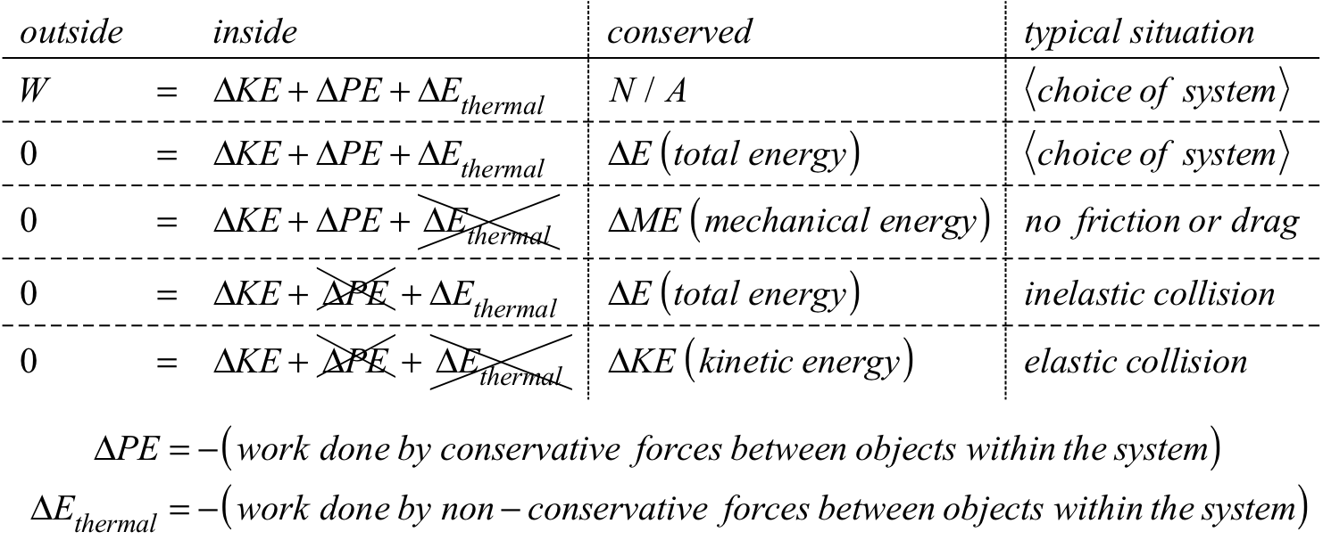
- The first entry allows for outside work to be done, which means that the system is not closed, and energy can enter or exit it via work done by force interactions with objects outside the system. We need to use this model when the statement of the problem does not let us isolate a closed system. In general we try to avoid it whenever possible, so that we don't have to perform any line integrals!
- The second entry assumes a closed system, which includes both conservative and non-conservative forces. The energy within this system can then change forms, but the total never changes.
- The third entry is a special case where there are no non-conservative forces within the closed system (or rather, the work done by the non-conservative forces is negligible). This is the model that features "frictionless surfaces" and "no air resistance."
- The fourth and fifth entries we will use a bit later. Suppose there are two objects in a closed system, which can only interact with each other, but the force has a limited range. When they are far apart, they don't interact. When they get close together, they push off one another, in what can be best described as a "collision," after which they are once again far enough apart that they don't interact. If one of the forces between the two objects is non-conservative, then some kinetic energy is converted to thermal, and even after the objects separate, this energy does not come back to kinetic form. In the case of conservative force interactions between the objects, however, the potential energy only depends upon the positions of the objects, and they end up in the same state after the collision as they were in before the collision (i.e. too far apart to interact), so for collisions we never have to take into account changes of potential energy. If the only forces present in a collision are conservative, then no thermal energy is produced, and the kinetic energy is conserved.
Now perhaps it is clear where “conservative” and “non-conservative” forces got their names – forces that conserve mechanical energy are conservative, and those that don’t are non-conservative.
Potential Energy Function for Gravity
It's all well-and-good to introduce all these models, but unless we have shortcuts for plugging into the conservation equations, we still have to perform work line integrals. The shortcuts we seek come from the presence of the potential energy changes. It is clearly much easier to compute the difference of two numbers as we would in the case of \(\Delta PE\) than it is to compute the work integral from scratch each time. So we will benefit from taking a few minutes to determine the potential energy functions for various conservative forces ahead of time, which we will then be able to use over and over. We start, as always, with gravity. In Equation 3.2.1, we computed the work done by the gravity force on a projectile, and found:
\[ W_{grav} \left( A \rightarrow B \right) = - mg \Delta y \]
Clearly mg remains constant, so relating this to the negative change of gravitational potential energy immediately gives:
\[ \Delta {PE}_{grav} = mg \Delta y \]
For reasons we will see later, it is helpful to define the potential energy due to gravity as a function of \(y\). When we get to this point, it's best to drop the two-letter "\(PE\)" in favor of a single-letter function. It is traditional to use \(U\). We therefore define:
\[ U \left( y \right) = mgy + U_o, \]
where \(U_o\) is an arbitrary constant. This constant comes about because if we take a difference of potential energies at two different altitudes, the constant drops out:
\[ \Delta U_{grav} = U \left( y_B \right) - U \left( y_A \right) = \left( mgy_B + U_o \right) - \left( mgy_A + U_o \right) = mg \left(y_B - y_A \right) = mg \Delta y \]
What this means is that we can reference the zero potential energy to be anywhere, and things will still always work out.
Alert
This last point bears repeating and expanding. Potential energy only has meaning inasmuch as it changes from one place to another. Remember, it came from work done by a conservative force, and defining work at a single point makes no sense. We can define a potential energy function that is defined by a number of joules at every point in space, but we can – without changing any physics – add or subtract a fixed number of joules from every position. in other words, we can call any position at all the point of "zero potential energy." Of course, once a position of zero potential energy is selected, the potential energy at every other point in space is fixed (we can't arbitrarily add or subtract a different constant value everywhere, or the \(\delta U's\) between points would also change.
Let's try this out for – you guessed it – the simplest example imaginable. Throw a rock straight up at some initial speed, starting at a height \(y_o\). How fast is it moving after it has risen to a height \(y_f\)? We are ignoring air resistance here, so we will use the mechanical energy conservation model, which only involves kinetic and potential energy. First, write down expressions for the kinetic and potential energy at the start and at the finish, then plug them into the conservation equation:
\[ \left. \begin{array}{l} initial: {KE}_i = \frac{1}{2}mv_i^2 \;\;\; U_{grav}\left(y_i\right) = mgy_i + U_o \\ final:\; {KE}_f = \frac{1}{2}mv_f^2 \;\;\; U_{grav}\left(y_f \right) = mgy_f + U_o \end{array} \right\} \;\; \Rightarrow \;\; 0 = \Delta KE + \Delta U_{grav} = \frac{1}{2}mv_f^2 - \frac{1}{2}mv_i^2 + mgy_f - mgy_i \;\;\; \Rightarrow \;\;\; v_f = \sqrt{v_i^2 - 2g\left( y_f - y_i \right)} \]
Sure enough, this result matches what we get using kinematics from Chapter 1. But notice that if the object had an \(x\)-component of velocity, then the velocity-squared in the kinetic energy includes another piece:
\[ \Delta KE = \frac{1}{2}mv_B^2 - \frac{1}{2}mv_A^2 = \frac{1}{2}m \left( v^2_{xB} + v^2_{yB} \right) - \frac{1}{2}m \left( v^2_{xA} + v^2_{yA} \right) \]
But of course the \(x\)-component of velocity never changes, so we end up with the same change in KE as before. Notice that we don't have to worry about vertical and horizontal components in this example, because we have confined ourselves to only looking at changes in speed, not direction.
Great, so our mechanical energy conservation model works for projectiles, but we already knew how to solve those. Now let’s look at something that is significantly harder to solve with Newton’s second law and kinematics.
Figure 3.4.2 – Loop-de-Loop
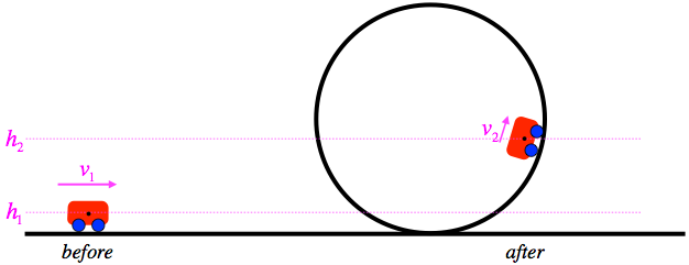
Our system here is the car (and the earth, so that work done by gravity is within the system), but the frictionless track is not included. This means that the normal force on the car by the track is a force coming from outside the system. But this doesn't mean we can't use a mechanical energy conservation model, because the normal force is at all times perpendicular to the motion. So while there is an outside force on the system, it doesn't do any work, which is what matters in our calculation. The car will change height and speed like a projectile, so we have precisely the same result as with the projectile, since it doesn’t matter how the car got from point A to point B – rolling on a track or flying through the air, and we get exactly the same result as above:
\[ v_2 = \sqrt{ v_1^2 - 2g\left( h_2 - h_1 \right)} \]
This required significantly less work than is involved using Newton's second law, and that is the point of constructing these energy conservation models. So long as we only want to know about the speed of the car and not its direction of motion or the time it takes to make its journey, this model gets us quickly to an answer. As an example of this lost information, change the final position of the car to the same height on the other side of the loop (on its way down after going around). The direction of the car's velocity is clearly different from the case above, and the time it took to get there is also different. All we can determine from this model is that the speeds are the same.
ExAmple \(\PageIndex{1}\)
There are few things as fun as swinging into a river from a rope swing tied to the limb of a tree on its banks. Suppose you are swinging on such a rope which has a length of 6.0m, and which hangs straight down to the shoreline with its open end 2.4m above the water level. You start your swing at rest from dry land with the rope at a 60º angle with the vertical, and release the rope at an angle of 30º with the vertical (over the water, obviously).
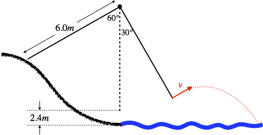
- Find your speed at the point when you release the rope.
- Find the distance above the water that you reach at the peak of your flight.
- Solution
-
a. The tension of the rope does no work here, as it acts perpendicular to your motion throughout. Ignoring air resistance, we therefore can use mechanical energy conservation to find the speed at the point of release. Let us will use as the zero potential energy reference point the tree branch. The distances below this reference point are easy to compute, as the length of the rope \(L\) is the hypotenuse for both triangles:
\[ \left. \begin{array}{l} starting \; height = y_o = -L \cos 60^o = -\dfrac{1}{2} L \\ ending \; height = y_f = -L \cos 30^o = - \dfrac{\sqrt{3}}{2} L \end{array} \right\} \;\;\; \Rightarrow \;\;\; \Delta U_{grav} = mg \left(y_f - y_o \right) = mgL \left( \dfrac{1 - \sqrt{3}}{2} \right) \nonumber \]
Putting this into mechanical energy conservation with a starting speed of zero gives us the final speed:
\[ 0 = \Delta KE + \Delta U_{grav} = \frac{1}{2} mv_f^2 - \frac{1}{2} mv_o^2 + mgL \left( \dfrac{1 - \sqrt{3}}{2} \right) \;\;\; \Rightarrow \;\;\; v_f = \sqrt{gL \left(\sqrt{3} - 1 \right)} = \boxed{6.6 \frac{m}{s}} \nonumber \]
b. We know that at the point of release, the velocity vector makes a 30º angle with the horizontal, so the horizontal component of this velocity (which never changes) is:
\[ v_x = v \cos 30^o = 5.6 \frac{m}{s} \nonumber \]
When you hit your peak height, you will have a zero \(y\)-component of velocity, so the quantity above will be your speed. You still have the same mechanical energy at this point as you had at the beginning, so we can compute how far below the tree limb you are at this point using mechanical energy conservation from the very beginning to the point where you reach the peak:
\[ 0 = \Delta KE + \Delta U_{grav} = \frac{1}{2} mv_f^2 - \frac{1}{2} mv_o^2 + mgy_{peak} - mgy_o \;\;\; \Rightarrow \;\;\; y_{peak} = y_o - \dfrac{v_f^2}{2g} = -4.7m \nonumber \]
This is measured from our \(y=0\) reference point at the tree branch, so since we know how high the tree branch is above the water, have:
\[ h = 6.0m + 2.4m - 4.7m = \boxed{3.7m} \]
Potential Energy Function for Elastic Force
For the mass on the spring we found:
\[ W_{spring} \left( A \rightarrow B \right) = - \frac{1}{2} k \Delta \left( x^2 \right) \]
If we go back to the calculation of the work done by a spring, we note the variable \(x\) is defined such that when it equals zero, the spring is in its equilibrium position.
As with the case of gravity, this immediately implies a function for elastic potential energy:
\[ \Delta PE_{elastic} = -W_{spring} \left( A \rightarrow B \right) \;\;\; \Rightarrow \;\;\; U_{elastic} \left( x \right) = \frac{1}{2}kx^2 +U_o \]
If we go back to the calculation of the work done by a spring, we note the variable \(x\) is defined such that when it equals zero, the spring is in its equilibrium position. But suppose we happen to define our coordinate system differently, with the spring in equilibrium at a position we'll call \(x_o\)? In this case we only need to make the substitution \(x \rightarrow x-x_o \), giving:
\[U_{elastic} \left( x \right) = \frac{1}{2}k \left(x-x_o \right)^2 + U_o \]
Example \(\PageIndex{2}\)
A ball is launched straight up into the air with the apparatus shown below. The ball is pushed upward so that it compresses the spring, and is released from rest. It then travels around a frictionless half-circle track, at the bottom of which is a scale that measures the contact force the ball exerts on the track at that point. The mass of the ball is \(m = 0.400kg\), the stiffness of the spring is \(k = 22.0 \frac{N}{m}\), and the radius of the track is 1.60m. When the ball passes over the scale, it reads 18.5N.
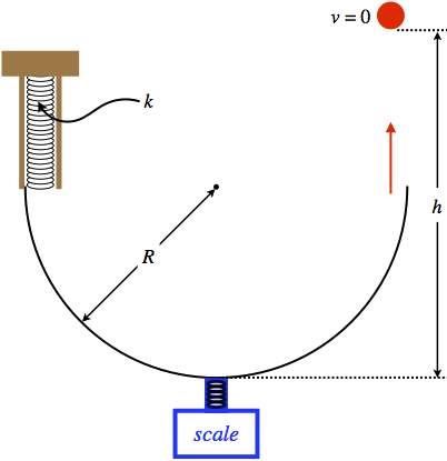
- Find the speed of the ball as it passes the scale.
- Find the height \(h\) reached by the ball.
- Find the amount that the spring was compressed before the ball was released.
- Solution
-
a. Start with a force diagram of the ball at the scale (gravity force down, normal force up), then use the facts that the scale measures the normal force and the ball's acceleration is centripetal:
\[ N - mg = ma_c = m \dfrac{v^2}{R} \;\;\; \Rightarrow \;\;\; v = \sqrt{R \left( \frac{N}{m} - g \right)} = 7.64 \frac{m}{s} \nonumber \]
b. There is no friction force by the track, and the contact force it exerts is perpendicular to the motion, so it does no work, which means that mechanical energy is conserved. With the speed of the ball at the bottom, we can therefore compute the height it reaches, where it comes to rest:
\[0 = \Delta KE + \Delta U_{grav} = \frac{1}{2} mv_f^2 - \frac{1}{2} mv_o^2 + mgh \;\;\; \Rightarrow \;\;\; h = \dfrac{v_o^2}{2g} = 2.98m \nonumber \]
c. We know the total energy in the system, either from the KE at the scale, or the PE at the peak height:
\[ E_{tot} = mgh = 11.7J \nonumber \]
When the ball compressed the spring, it had no KE, so all of this energy was stored in the PE of gravity and the elastic PE of the spring. Calling the compression \(\Delta y\), then the height of the ball at the start is \(R+\Delta y\). Summing the two PE’s and setting the sum equal to the total energy gives a quadratic equation, which we then solve for \(\Delta y\):
\[ E_{tot} = mg \left(R+\Delta y \right) +\frac{1}{2}k\left(\Delta y\right)^2 \;\;\; \Rightarrow \;\;\; \Delta y = \dfrac{-mg \pm \sqrt{\left(mg\right)^2 - 2k\left(mgR-E_{tot}\right)}}{k} = \boxed{0.55m} \nonumber \]