2.12: Applications of Newton's Equations of Motion

Newton’s equation of motion can be written in the form

\[ \label{eq:2.90} \mathbf{F} = \frac{d\mathbf{p}}{dt} = m\frac{d\mathbf{v}}{dt} = m\frac{d^2\mathbf{r}}{dt^2}  \]

A description of the motion of a particle requires a solution of this second-order differential equation of motion. This equation of motion may be integrated to find r(t) and v(t) if the initial conditions and the force field F(t) are known. Solution of the equation of motion can be complicated for many practical examples, but there are various approaches to simplify the solution. It is of value to learn efficient approaches to solving problems.

The following sequence is recommended

a) Make a vector diagram of the problem indicating forces, velocities, etc.

b) Write down the known quantities.

c) Before trying to solve the equation of motion directly, look to see if a basic conservation law applies. That is, check if any of the three first-order integrals, can be used to simplify the solution. The use of conservation of energy or conservation of momentum can greatly simplify solving problems.

The following examples show the solution of typical types of problem encountered using Newtonian mechanics

2.12.1 Constant force problems

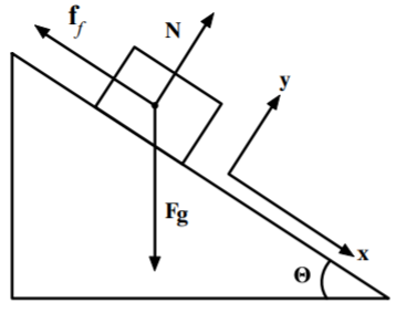
Problems having a constant force imply constant acceleration. The classic example is a block sliding on an inclined plane, where the block of mass m is acted upon by both gravity and friction. The net force F is given by the vector sum of the gravitational force \(\mathbf{F}_g \), normal force \( \mathbf{N}\) and frictional force \( \mathbf{f}_f \)

\[ \label{eq:2.91} \mathbf{F} = \mathbf{F}_g + \mathbf{N + f}_f  = \mathbf{a} \]

Taking components perpendicular to the inclined plane in the y direction

\[ \label{eq:2.92} -F_g \cos \theta + N = 0 \]

Figure 2.3: Block on an inclined plane

That is, since \( F_g = mg \)

\[ \label{eq:2.93} N = mg \cos \theta \]

Similarly, taking components along the inclined plane in the y direction

\[ \label{eq:2.94} F_g \sin \theta - f_f = m \frac{d^2 x}{dt^2} \]

 

Using the concept of coefficient of friction \( \mu \)

\[ \label{eq:2.95} f_f = \mu N \]

Thus the equation of motion can be written as

\[ \label{eq:2.96} mg( \sin \theta - \mu \cos \theta ) = m \frac{d^2 x}{dt^2} \]

The block accelerates if \( \sin \theta > \mu \cos \theta \), that is, \(\tan \theta > \mu \). The acceleration is constant if \( \mu \) and \( \theta \) are constant, that is

\[ \label{eq:2.97} \frac{d^2x}{dt^2} = g ( \sin \theta - \mu \cos \theta ) \]

Remember that if the block is stationary, the friction coefficient balances such that \( ( \sin \theta - \mu \cos \theta ) = 0 \) that is, \( \tan \theta = \mu \). However, there is a maximum static friction coefficient \( \mu _S \) beyond which the block starts sliding. The kinetic coefficient of friction \( \mu_K \) is applicable for sliding friction and usually \( \mu_K < \mu_S \) Another example of constant force and acceleration is motion of objects free falling in a uniform gravitational field when air drag is neglected. Then one obtains the simple relations such \( v = u + at \), etc.

2.12.2 Linear Restoring Force

An important class of problems involve a linear restoring force, that is, they obey Hooke’s law. The equation of motion for this case is

\[ \label{eq:2.98} F ( x ) = -kx = m \ddot{x} \]

It is usual to define

\[ \label{eq:2.99} \omega_0 ^2 \equiv \frac{k}{m} \]

Then the equation of motion then can be written as

\[ \label{eq:2.100} \ddot{x} + \omega_0^2 x = 0 \]

which is the equation of the harmonic oscillator. Examples are small oscillations of a mass on a spring, vibrations of a stretched piano string, etc. The solution of this second order equation is

\[ \label{eq:2.101} x(t) = A \sin ( \omega _0 t - \delta ) \]

This is the well known sinusoidal behavior of the displacement for the simple harmonic oscillator. The angular frequency \( \omega_0 \)

\[ \label{eq:2.102} \omega_0 = \sqrt{\frac{k}{m}} \]

Note that for this linear system with no dissipative forces, the total energy is a constant of motion as discussed previously. That is, it is a conservative system with a total energy E given by

\[ \label{eq:2.103} \frac{1}{2} m \dot{x} ^2 + \frac{1}{2} kx ^2 = E \]

The first term is the kinetic energy and the second term is the potential energy. The Virial theorem gives that for the linear restoring force the average kinetic energy equals the average potential energy.

2.12.3 Position-dependent conservative forces

The linear restoring force is an example of a conservative field. The total energy E is conserved, and if the field is time independent, then the conservative forces are a function only of position. The easiest way to solve such problems is to use the concept of potential energy U illustrated in Figure 2.4.

\[ \label{eq:2.104} U_2 - U_1 = - \int_1^2 \mathbf{F} \cdot d \mathbf{x} \]

Consider a conservative force in one dimension. Since it was shown that the total energy \( E = T + U \) is conserved for a conservative field, then

\[\label{2.105} E = T + U = \frac{1}{2} mv^2 + U  (x) \]

Therefore:

\[\label{2.106} v = \frac{dx}{dt} = \pm \sqrt{\frac{2}{m} [ E - U (x) ] }  \]

Integration of this gives

\[\label{2.107} t - t_0 = \int_{x_0}^x \frac{\pm dx}{\sqrt{\frac{2}{m} [ E - U (x) ]}}\]

where \( x = x_0 \) when \( t = t_0 \) Knowing \( U(x) \) it is possible to solve this equation as a function of time.

Figure 2.4: One-dimensional potential WIP

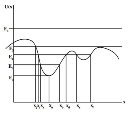
It is possible to understand the general features of the solution just from inspection of the function \( U(x) \). For example, as shown in figure 2.4 the motion for energy \( E_1 \) is periodic between the turning points \( x_a \) and \(x_b\). Since the potential energy curve is approximately parabolic between these limits the motion will exhibit simple harmonic motion. For \( E_0 \) the turning point coalesce to \( x_0 \) that is there is no motion. For total energy \( E_2 \) the motion is periodic in two independent regimes, \( x_c \leq x \leq x_d \) and \( x_e \leq x \leq f \). Classically the particle cannot jump from one pocket to the other. The motion for the particle with total energy \( E_3 \) is that it moves freely from infinity, stops and rebounds at \( x = x_g \) and then returns to infinity. That is the particle bounces off the potential at \( x_g \). For energy \( E _4 \) the particle moves freely and is unbounded. For all these cases, the actual velocity is given by the above relation for \( v (x) \). Thus the kinetic energy is largest where the potential is deepest. An example would be motion of a roller coaster car.

Position-dependent forces are encountered extensively in classical mechanics. Examples are the many manifestations of motion in gravitational fields, such as interplanetary probes, a roller coaster, and automobile suspension systems. The linear restoring force is an especially simple example of a position-dependent force while the most frequently encountered conservative potentials are in electrostatics and gravitation for which the potentials are;

\[ \label{eq:ElecPot} \nonumber \tag{Electrostatic Potential energy} U(r) = \frac{1}{4 \pi \epsilon _0} \frac{q_1 q_2}{r_{12}^2} \]

\[ \label{eq:GravPot} \nonumber \tag{Gravitational Potential energy} U(r) = -G  \frac{m_1 m_2}{r_{12}^2} \]

Knowing \( U (r) \) it is possible to solve the equation of motion as a function of tim

2.7 Example: Diatomic molecule

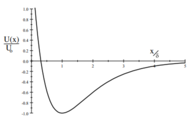
An example of a conservative field is a vibrating diatomic molecule which has a potential energy dependence with separation distance x that is described approximately by the Morse function

\[ \nonumber U(x) = U_0 \Big [ 1 - e^{ - \frac{ ( x - x_0 )}{ \delta }} \Big ] ^2 - U_0 \]

where \( U_0, x_0 \ and \ \delta \) are parameters chosen to best describe the particular pair of atoms. The restoring force is given by

\[ \nonumber F(x) = - \frac{dU(x)}{dx} =  2 \frac{U_0}{ \delta } \Big [ 1 - e^{- \frac{ ( x - x_0 )}{ \delta }} \Big ]  \Big [  e^{- \frac{ ( x - x_0 )}{ \delta }} \Big ] \]

This has a minimum value of \( U (x_0) = U_0 \) at \( x = x_0 \).

 figure - potential energy function (WIP)

Note that for small amplitude oscillations, where

\[ \nonumber ( x - x_0 ) < < \delta \]

the exponential term in the potential function can be expanded to give

\[ \nonumber U(x) \approx U_0 \Bigg [ 1 - (1 - -\frac{ (x - x_0 )}{ \delta}) \Bigg ] ^2 - U_0 \approx \frac{U_0}{\delta ^2} ( x - x_0 ) ^2 - U_0 \]

This gives a restoring force

\[ \nonumber F(x) = - \frac{dU(x)}{dx} = - 2 \frac{U_0}{ \delta} ( x - x_0 ) \]

That is, for small amplitudes the restoring force is linear.

2.12.4 Constrained Motion

A frequently encountered problem with position dependent forces is when the motion is constrained to follow a certain trajectory. Forces of constraint must exist to constrain the motion to a specific trajectory. Examples are, the roller coaster, a rolling ball on an undulating surface, or a downhill skier, where the motion is constrained to follow the surface or track contours. The potential energy can be evaluated at all positions along the constrained trajectory for conservative forces such as gravity. However, the additional forces of constraint that must exist to constrain the motion, can be complicated and depend on the motion. For example, the roller coaster must always balance the gravitational and centripetal forces. Fortunately forces of constraint \( \mathbf{F}_C \) often are normal to the direction of motion and thus do not contribute to the total mechanical energy since then the work done \( \mathbf{F} _C \cdot d \mathbf{l} \) is zero. Magnetic forces F =qv × B exhibit this feature of having the force normal to the motion.

Solution of constrained problems is greatly simplified if the other forces are conservative and the forces of constraint are normal to the motion, since then energy conservation can be used.

2.8 Example: Roller coaster

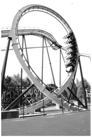
Consider motion of a roller coaster shown in the adjacent figure. This system is conservative if the friction and air drag are neglected and then the forces of constraint are normal to the direction of motion. The kinetic energy at any position is just given by energy conservation and the fact that

\[ \nonumber E = T + U \]

where U depends on the height of the track at any the given location. The kinetic energy is greatest when the potential energy is lowest. The forces of constraint can be deduced if the velocity of motion on the track is known. Assuming that the motion is confined to a vertical plane, then one has a centripetal force of constraint \( \frac{mv^2}{ \rho } \) normal to the track inwards towards the center of the radius of curvature \( \rho \), plus the gravitation force downwards of mg.

The constraint force is \( \frac{mv^2_T}{ \rho } - mg \) upwards at the

top of the loop, while it is \( \frac{mv^2_B}{ \rho } + mg\) downwards at the bottom of the loop. To ensure that the car and occupants do not leave the required trajectory, the force upwards at the top of the loop has to be positive, that is, \(  v^2_T \geq \rho g \). The velocity at the bottom of the loop is given by \( \frac{1}{2} m v^2_B = \frac{1}{2}mv_T^2 + 2mg \rho \) assuming that the track has a constant radius of curvature \( \rho \). That is; at a minimum \( v^2 _B = \rho g + 4 \rho g = 5 \rho g \) Therefore the occupants now will feel an acceleration downwards of at least \( \frac{v^2_B}{\rho} + g = 6g \) at the bottom of the loop. The first roller coaster was built with such a constant radius of curvature but an acceleration of 6g was too much for the average passenger. Therefore roller coasters are designed such that the radius of curvature is much larger at the bottom of the loop, as illustrated, in order to maintain sufficiently low g loads and also ensure that the required constraint forces exist.

Note that the minimum velocity at the top of the loop, \( v_T \), implies that if the cart starts from rest it must start at a height \( h \geq \frac{\rho}{2} \) above the top of the loop if friction is negligible. Note that the solution for the rolling ball on such a roller coaster differs from that for a sliding object since one must include the rotational energy of the ball as well as the linear velocity. Looping the loop in a glider involves the same physics making it necessary to vary the elevator control to vary the radius of curvature throughout the loop to minimize the maximum g load.

2.12.5 Velocity Dependent Forces

Velocity dependent forces are encountered frequently in practical problems. For example, motion of an object in a fluid, such as air, where viscous forces retard the motion. In general the retarding force has a complicated dependence on velocity. The drag force usually is expressed in terms of a drag coefficient

\[ \label{eq:2.108} \mathbf{F}_D(v) = -\frac{1}{2} c_D \rho A v^2 \mathbf{\hat{v}} \]

where \( c_D \) is a dimensionless drag coefficient, \( \rho \) is the density of air, \( A \) is the cross sectional area perpendicular to the direction of motion, and \( v \) is the velocity. Modern automobiles have drag coefficients as low as 0.3. As described in chapter 4, the drag coefficient \( c_D \) depends on the Reynold’s number which relates the inertial to viscous drag forces. Small sized objects at low velocity, such as light raindrops, have low Reynold’s numbers for which \( c_D \) is roughly proportional to \( v^{-1} \) leading to a linear dependence of the drag force on velocity, i.e. \( F_D (v) \propto v \). Larger objects moving at higher velocities, such as a car or sky-diver, have higher Reynold’s numbers for which \( c_D \) is roughly independent of velocity leading to a drag force \( F_D (v) \propto v^2 \). This drag force always points in the opposite direction to the unit velocity vector. Approximately for air

\[ \label{eq:2.109} \mathbf{F}_D(v) = -(c_1v + c_2 v^2 ) \hat{v} \]

where for spherical objects of diameter\( D, c_1 \approx 1.55 \times 10^{-4} D \) and \( c_2 \approx 0.22D^2 \) and in MKS units. Fortunately, the equation of motion usually can be integrated when the retarding force has a simple power law dependence. As an example, consider free fall in the Earth’s gravitational field.

2.9 Example: Vertical fall in the Earth's gravitational field.

Linear regime \( c_1 > > c_2 v \) 

For small objects at low-velocity, i.e. low Reynold’s number, the drag has approximately a linear dependence on velocity. The equation of motion is

\[ \nonumber -mg -c_1 v =m \frac{dv}{dt} \]

Separate the variables and integrate

\[ \nonumber t = \int_{v_0}^v \frac{m dv}{-mg - c_1 v } = -\frac{m}{c_1} ln \bigg ( \frac{mg + c_1 v}{mg + c_1v_0} \bigg ) \]

That is

\[ \nonumber v = -\frac{mg}{c_1} + \bigg ( \frac{mg}{c_1} + v_0 \bigg ) e^{-\frac{c_1}{m} t} \]

Note that for \( t  \gg \frac{m}{c_1} \) the velocity approaches a terminal velocity of \( v_\infty = -\frac{mg}{c_1}  \). The characteristic time constant is \( \tau = \frac{m}{c_1} = \frac{v_\infty}{g} \). Note that if \( v_0 = 0 \), then

\[ \nonumber v  = v_\infty \Big ( 1 - e^{-\frac{t}{\tau}} \Big ) \]

For the case of small raindrops with \( D = 0.5 mm \) then \( v_\infty = 8 \ m/s \ (18 \ mph) \) and time constant \( \tau = 0.8 s \). Note that in the absence of air drag, these rain drops falling from 2000 m would attain a velocity of over 400 mph. It is fortunate that the drag reduces the speed of rain drops to non-damaging values. Note that the above relation would predict high velocities for hail. Fortunately, the drag increases quadratically at the higher velocities attained by large rain drops or hail, and this limits the terminal velocity to moderate values. As known in the mid-west, these velocities still are sufficient to do considerable crop damage.

Quadratic regime  \( \hspace{4 cm} c_2v > > c_1 \)

For larger objects at higher velocities, i.e. high Reynold’s number, the drag depends on the square of the velocity making it necessary to differentiate between objects rising and falling. The equation of motion is

\[ \nonumber -mg \pm c_2v^2 = m\frac{dv}{dt} \]

where the positive sign is for falling objects and negative sign for rising objects. Integrating the equation of motion for falling gives

\[ \nonumber t = \int_{v_0}^v \frac{mdv}{-mg + c_2v^2} = \tau \bigg ( tanh^{-1} \frac{v_0}{v_\infty} - tanh^{-1} \frac{v}{v_\infty} \bigg ) \]

where \( \tau = \sqrt{\frac{m}{c_2g}} \) and \( v_\infty = \sqrt{\frac{mg}{c_2}} \) That is, \( \tau = \frac{v_\infty}{g} \) For the case of a falling object with \( v_0 = 0 \) solving for velocity gives

\( v = v_\infty tanh \frac{t}{ \tau} \)

As an example, a 0.6 kg basket ball with D = 0.25 m will have \( v_\infty = 20 m/s \) ( 43 mph) and \( \tau = 2.1 \ s \).

Consider President George H.W. Bush skydiving. Assume his mass is 70 kg and assume an equivalent spherical shape of the former President to have a diameter of \( D = 1 \ m \) This gives that \( v_\infty = 56 \ m/s \) ( 120 mph) and \( \tau = 5.6 \ s \). When Bush senior opens his 8 m diameter parachute his terminal velocity is estimated to decrease to 7m/s ( 15 mph) which is close to the value for a typical ( 8m) diameter emergency parachute which has a measured terminal velocity of 11 mph in spite of air leakage through the central vent needed to provide stability.

2.10 Example: Projectile motion in air

Consider a projectile initially at x = y = 0, at t = 0, that is fired at an initial velocity v\( v_0 \) at an angle \( \theta \) to the horizontal. In order to understand the general features of the solution, assume that the drag is proportional to velocity. This is incorrect for typical projectile velocities, but simplifies the mathematics. The equations of motion can be expressed as

\[ \nonumber m \ddot{x} = - km \ddot{x} \]

\[ \nonumber m \ddot{y} = - km \dot{y} - mg \]

where k is the coefficient for air drag. Take the initial conditions at t = 0 to be x = y = 0, \( \dot{x} = v_0 \cos \theta, \dot{y} = v_0 \sin \theta \).

Solving in the x coordinate,

\[ \nonumber \frac{ d\mathbf{x} }{dt} = -k \dot{x} \]

Therefore

\[ \nonumber \dot{x} = v_0 \cos \theta e ^{-kt} \]

That is, the velocity decays to zero with a time constant \( \tau = \frac{1}{k} \)

Integration of the velocity equation gives

\[ \nonumber x = \frac{v_0}{k} ( 1 - e ^{-kt} ) \]

Note that this implies that the body approaches a value of  \( x  =\frac{v_0}{k} \) as \( t \rightarrow \infty \)

The trajectory of an object is distorted from the parabolic shape, that occurs for k = 0, due to the rapid drop in range as the drag coefficient increases. For realistic cases it is necessary to use a computer to solve this numerically.

2.12.6 Systems with Variable Mass

Classic examples of systems with variable mass are the rocket, nuclear fission and other modes of nuclear decay.

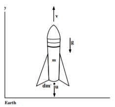
Consider the problem of rocket motion in a gravitational field. When there is a vertical gravitational external field the vertical momentum is not conserved due to both gravity and the ejection of rocket propellant. In a time dt the rocket ejects propellant \(dm_p \) with exhaust velocity relative to the rocket of u. Thus the momentum imparted to this propellant is

\[ \label{eq:2.110} dp_p = -udm_p \]

Therefore the rocket is given an equal and opposite increase in momentum

\[\label{eq:2.111} dp_R = +udm_p \]

In the time interval dt the net change in the linear momentum of the rocket plus fuel system is given by

\[ \label{eq:2.112} dp = (m - dm_p ) ( v + dv) + dm_p (v - u ) - mv = mdv - udm_p \]

The rate of change of the linear momentum thus equals

\[\nonumber F_{ex} = \frac{dp}{dt} = m\frac{dv}{dt} - u \frac{dm_p}{dt} \]

Consider the problem for the special case of vertical ascent of the rocket against the external gravitational force \( F_{ex} = -mg \). Then

\[ \label{eq:2.113} -mg + u\frac{dm_p}{dt} = m\frac{dv}{dt} \]

This can be rewritten as

\[ \label{eq:2.114} -mg + u\dot{m}_p = m\dot{v} \]

 Figure 2.5: Vertical motion of a rocket in a gravitational field (WIP)

The second term comes from the variable mass. But the loss of mass of the rocket equals the mass of the ejected propellant. Assuming a constant fuel burn \( \dot{m}_p = \alpha \) then

\[ \label{eq:2.115} \dot{m} = -\dot{m}_p = -\alpha \]

where \( \alpha > 0 \) Then the equation becomes

\[ \label{eq:2.116} dv = \big ( -g + \frac{ \alpha}{m} u \big ) dt \]

Since

\[ \label{eq:2.117} \frac{dm}{dt} = -\alpha \]

then

\[\label{eq:2.118} - \frac{dm}{\alpha} = dt \]

Inserting this in the above equation gives

\[ \label{eq:2.119} dv = \big ( \frac{g}{\alpha} - \frac{u}{m} \big ) dm \]

Integration gives

\[ \label{eq:2.120} v = - \frac{g}{\alpha} ( m_0 - m ) + u \ln \big ( \frac{m_0}{m} \big ) \]

But the change in mass is given by

\[ \label{eq:2.121} \int_{m_0}^m dm = - \alpha \int_0^t dt \]

That is

\[ \label{eq:2.122} m_0 - m = \alpha t \]

Thus

\[ \label{eq:2.123} v = -gt  + u \ln \big ( \frac{m_0}{m} \big ) \]

Note that once the propellant is exhausted the rocket will continue to fly upwards as it decelerates in the gravitational field. You can easily calculate the maximum height. Note that this formula assumes that the acceleration due to gravity is constant whereas for large heights above the Earth it is necessary to use the true gravitational force \( - G \frac{Mm}{r^2} \) where r is the distance from the center of the earth. In real situations it is necessary to include air drag which requires use of a computer to numerically solve the equations of motion. The highest rocket velocity is attained by maximizing the exhaust velocity and the ratio of initial to final mass. Because the terminal velocity is limited by the mass ratio, engineers construct multistage rockets that jettison the spent fuel containers and rockets.

2.12.7 Rigid-body rotation about a body-fixed rotation axis

The most general case of rigid-body rotation involves rotation about some body-fixed point with the orientation of the rotation axis undefined. For example, an object spinning in space will rotate about the center of mass with the rotation axis having any orientation. Another example is a child’s spinning top which spins with arbitrary orientation of the axis of rotation about the pointed end which touches the ground about a static location. Such rotation about a body-fixed point is complicated and will be discussed in chapter 11. Rigid-body rotation is easier to handle if the orientation of the axis of rotation is fixed with respect to the rigid body. An example of such motion is a hinged door.

For a rigid body rotating with angular velocity \( \omega \) the total angular momentum L is given by

\[ \label{eq:2.124} \mathbf{L} = \sum_i^n \mathbf{L}_i = \sum_i^n \mathbf{r}_i \times \mathbf{p}_i \]

For rotation equation appendix D29 gives

\[ \nonumber \tag{2.94} \mathbf{v}_i = \mathbf{ \omega} \times \mathbf{r}_i \]

thus the angular momentum can be written as

\[ \label{eq:2.125} = \sum_i^n \mathbf{r}_i \times \mathbf{p}_i = \sum_i^n m_i \mathbf{r}_i \times \mathbf{\omega} \times \mathbf{r}_i \]

This can be simplified using the vector identity equation B.24 giving

\[ \label{eq:2.126} \mathbf{L} = \sum_i^n [ \big ( m_i r_i ^2 \big ) \mathbf{ \omega} - ( \mathbf{r}_i \cdot \mathbf{\omega} ) m_i \mathbf{r}_i ] \]

Rigid-body rotation about a body-fixed symmetry axis

The simplest case for rigid-body rotation is when the body has a symmetry axis with the angular velocity \( \mathbf{\omega} \) parallel to this body-fixed symmetry axis. For this case then \( \mathbf{r}_i \) can be taken perpendicular to \( \mathbf{\omega} \) for which the second term in equation 2.126, i.e. \( \mathbf{r}_i \cdot \omega  = 0\), thus

\[ \nonumber \label{RigidBody} \tag{ \( \mathbf{r}_i \ perpendicular \ to \ \mathbf{\omega}\)} \mathbf{L}_{sym } = \sum_i^n \big ( m_ir_i^2 \big ) \omega \]

The moment of inertia about the symmetry axis is defined as

\[ \label{eq:2.127} I_{sym} = \sum_i^n m_ir_u^2 \]

where \( r_i \) is the perpendicular distance from the axis of rotation to the body, \( m_i \) For a continuous body the moment of inertia can be generalized to an integral over the mass density \rho of the body

\[ \label{eq:2.128} I_{sym} = \int \rho r^2 dV \]

where \( r \) is perpendicular to the rotation axis. The definition of the moment of inertia allows rewriting the angular momentum about a symmetry axis \( \mathbf{L}_{sym} \) in the form

\[ \label{eq:2.129} \mathbf{L}_{sym} = I_{sym}\mathbf{\omega} \]

where the moment of inertia \( I_{sym} \) is taken about the symmetry axis and assuming that the angular velocity of rotation vector is parallel to the symmetry axis.

Rigid-body rotation about a non-symmetric body-fixed axis

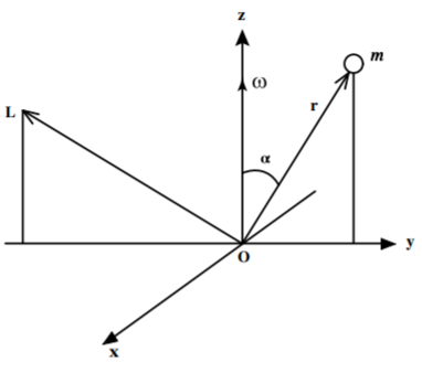
In general the fixed axis of rotation is not aligned with a symmetry axis of the body, or the body does not have a symmetry axis, both of which complicate the problem. For illustration consider that the rigid body comprises a system of \( n \) masses \( m_i \) located at positions \( \mathbf{r} \) with the rigid body rotating about the \( z \) axis with angular velocity \( \mathbf{\omega} \) That is,

\[ \label{eq:2.130} \mathbf{\omega} = \omega_z \hat{\mathbf{z}} \]

In cartesian coordinates the fixed-frame vector for particle i is

\[ \label{eq:2.131} \mathbf{r}_i = ( x_i, y_i, z_i ) \]

using these in the cross product (2.94) gives

\[ \label{eq:2.132} \mathbf{v}_i = \mathbf{\omega} \times \mathbf{r}_i = \begin{pmatrix} -\omega_z y_i \\ \omega_z x_i \\ 0 \end{pmatrix} \]

which is written as a column vector for clarity. Inserting \( \mathbf{v}_i \) in the cross-product \( \mathbf{r}_i \times \mathbf{v}_i \) gives the components of the angular momentum to be

\[ \nonumber \sum_i^n m_i \mathbf{r}_i \times \mathbf{v}_i \sum_i^n m_i \omega_z \begin{pmatrix} -z_ix_i \\ -z_iy_i \\ x_i^2 + y_i^2 \end{pmatrix} \]

Figure 2.6 (WIP)

That is, the components of the angular momentum are

\[ \label{eq:2.133} \begin{align*} L_x & = & - \bigg ( \sum_i^n m_i z_i x_i \bigg ) \omega_z \equiv I_{xz} \omega_z \\ L_y & = &  - \bigg ( \sum_i^n m_i z_i y_i \bigg ) \omega_z \equiv I_{yz} \omega_z \\ L_z & = & - \bigg ( \sum_i^n m_i [ x_i^2 + y_i^2 ]  \bigg ) \omega_z \equiv I_{xz} \omega_z \end{align*} \]

 

Note that the perpendicular distance from the z axis in cylindrical coordinates is \( \rho = \sqrt{x_i^2 y_i^2} \) thus the angular momentum \( L_z \) about the z axis can be written as

\[ \label{eq:2.134} L_z = \bigg ( \sum_i^n m_i \rho^2 \bigg ) \omega _z = I _{zz} \omega_z \]

where (2.134) gives the elementary formula for the moment of inertia \( I_{zz} = I_{sym} \) about the z axis given earlier in (2.129). The surprising result is that \( L_x \) and \( L_y \) are non-zero implying that the total angular momentum vector L is in general not parallel with \( \mathbf{\omega} \) This can be understood by considering the single body m shown in figure 2.6. When the body is in the \( y, z \) plane then x = 0 and \( L_x = 0 \) Thus the angular momentum vector L has a component along the −y direction as shown which is not parallel with ω and, since the vectors \( \mathbf{ \omega, L, r}_i \) are coplanar, then L must sweep around the rotation axis ω to remain coplanar with the body as it rotates about the \( \omega \) axis. Instantaneously the velocity of the body \( v_i \) is into the plane of the paper and, since \( \mathbf{L}_i = m_i\mathbf{r}_i \times \mathbf{v}_i \), then \mathbf{L}_i is at an angle (90^\circ − \alpha) to the z axis. This implies that a torque must be applied to rotate the angular momentum vector. This explains why your automobile shakes if the rotation axis and symmetry axis are not parallel for one wheel.

The first two moments in (2.133) are called products of inertia of the body designated by the pair of axes involved. Therefore, to avoid confusion, it is necessary to define the diagonal moment, which is called the moment of inertia, by two subscripts as \( I_{zz} \) Thus in general, a body can have three moments of inertia about the three axes plus three products of inertia. This group of moments comprise the inertia tensor which will be discussed further in chapter 11. If a body has an axis of symmetry along the z axis then the summations will give \( I_{xz} = I_{yz} = 0 \) while \( I_{zz} \) will be unchanged. That is, for rotation about a symmetry axis the angular momentum and rotation axes are parallel. For any axis along which the angular momentum and angular velocity coincide is called a principal axis of the body

2.11 Example: Moment of inertia of a thin door

Consider that the door has width a and height b and assume the door thickness is negligible with areal density \(\sigma kg/m^2 \). Assume that the door is hinged about the y axis. The mass of a surface element of dimension \( dx \cdot dy \) at a distance x from the rotation axis is \( dm = \sigma dx dy \) thus the mass of the complete door is \( M = \sigma a b \). The moment of inertia about the y axis is given by

\[ \nonumber I = \int_{x=0}^a \int_{y = 0}^b \sigma x^2 dydx = \frac{1}{3} \sigma b a^3 = \frac{1}{3} M a^2 \]

2.12 Example: Merry-go-round

A child of mass m jumps onto the outside edge of a circular merry-go-round of moment of inertia I, and radius R and initial angular velocity \( \omega_0 \) What is the final angular velocity \( \omega _f \) ? If the initial angular momentum is \( L_0 \) and, assuming the child jumps with zero angular velocity, then the conservation of angular momentum implies that

\[ \begin{align*} L_0 & = & L_f \\ I\omega_0 & = & I_\omega + mv_fR \\ I \frac{v_0}{R} & =& \frac{v_f}{R} ( I + mR^2 ) \end{align*} \]

That is

\[ \frac{v_f}{v_0} = \frac{\omega_f}{\omega_0} = \frac{I}{I + mR^2} \]

Note that this is true independent of the details of the acceleration of the initially stationary child.

2.13 Example: Cue pushes a billiard ball

 

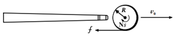
Consider a billiard ball of mass M and radius R is pushed by a cue in a direction that passes through the center of gravity such that the ball attains a velocity \( v_0 \). The friction coefficient between the table and the ball is \( \mu ). How far does the ball move before the initial slipping motion changes to pure rolling motion? Since the direction of the cue force passes through the center of mass of the ball, it contributes zero torque to the ball. Thus the initial angular momentum is zero at t = 0. The friction force f points opposite to the direction of motion and causes a torque \( N_s \) about the center of mass in the direction \( \hat{s} \)

\[ \nonumber \mathbf{N} = \mathbf{f} \cdot \mathbf{R} = \mu M g R \]

Since the moment of inertia about the center of a uniform sphere is \( I  =\frac{2}{5}MR^2 \) then the angular acceleration of the ball is

\[ \nonumber \tag{\( \alpha \)} \dot{\omega} = \frac{\mu M g R}{I} = \frac{ \mu M g R}{\frac{2}{5} MR ^2} = \frac{5}{2} \frac{\mu g}{R} \]

Moreover the frictional force causes a deceleration \( a_s \) of the linear velocity of the center of mass of

\[ \nonumber \tag{\( \alpha \)} a_s = - \frac{f}{M} = - \mu g \]

Integrating  \( \alpha \) from time zero to t gives

\[ \nonumber \omega = \int_0^t \dot{\omega} dt = \frac{5}{2} \frac{ \mu g}{R} t \]

The linear velocity of the center of mass at time t is given by integration of equation \( \beta \)

\[ \nonumber v_s = \int_0^t a_s dt = v_0 - \mu gt \]

The billiard ball stops sliding and only rolls when \( v_s = \omega R \), that is, when

\[ \nonumber \frac{5}{2} \frac{\mu g }{R} tR = v_0 - \mu gt \]

That is, when

\[ \nonumber t_{roll} = \frac{2}{7} \frac{v_0}{\mu g} \]

Thus the ball slips for a distance

\[ \nonumber s = \int_0^{t_{roll}} v_s dt = v_0 t_{roll} - \frac{\mu gt_{roll}^2}{2} = \frac{12}{49} \frac{v_0^2}{\mu g } \]

Note that if the ball is pushed at a distance h above the center of mass, besides the linear velocity there is an initial angular momentum of

\[ \omega = \frac{M v_0 h }{ \frac{2}{5} MR^2} = \frac{5}{2} \frac{v_o h}{R^2} \]

For the case \( h = \frac{2}{5} R \) then the ball immediately assumes a pure non-slipping roll. For \( h < \frac{2}{5} R \) one has \( \omega < \frac{v_0}{R} \) while \( h > \frac{2}{5} R \) corresponds to \( \omega > \frac{v_0}{R} \). In the latter case the frictional force points forward.

2.12.8 Time dependent forces

Many problems involve action in the presence of a time dependent force. There are two extreme cases that are often encountered. One is an impulsive force that acts for a very short time, for example, striking a ball with a bat, or the collision of two cars while the second force is an oscillatory time dependent force. The response to impulsive forces is discussed below whereas the response to oscillatory time dependent forces is discussed in chapter 3. Translational impulsive forces An impulsive force acts for a very short time relative to the response time of the mechanical system being discussed. In principle the equation of motion can be solved if the complicated time dependence of the force, F(t) is known. However, often it is possible to use the much simpler approach employing the concept of an impulse and the principle of the conservation of linear momentum. Define the linear impulse to be the first-order time integral of the time-dependent force.

\[ \label{eq:2.135} \mathbf{P} = \int \mathbf{F} (t) dt \]

Since \( \mathbf{F} (t) = \frac{d\mathbf{p}}{dt} \) then equation 2.135 gives that

\[ \label{eq:2.136} \mathbf{P} = \int_0^t \frac{d\mathbf{p}}{dt^\prime}dt^\prime = \int_0^t d\mathbf{p} =\mathbf{p}(t) - \mathbf{p}_0 = \Delta \mathbf{p} \]

Thus the impulse P is an unambiguous quantity that equals the change in linear momentum of the object that has been struck which is independent of the details of the time dependence of the impulsive force. Computation of the spatial motion still requires knowledge of F(t) since the 2.136 can be written as

\[ \label{eq:2.137} \mathbf{v}(t) = \frac{1}{m} \int_0^t \mathbf{F}(t^\prime) dt^\prime + \mathbf{v}_0 \]

Integration gives

\[ \label{eq:2.138} \mathbf{r}(t) - \mathbf{r}_0 = \mathbf{v}_0 t + \int_0^t \Bigg [ \frac{1}{m} \int_0^{\prime \prime} \mathbf{F} (t^\prime ) dt^\prime \Bigg ] dt^{\prime \prime } \]

In general this is complicated. However, for the case of a constant force \( \mathbf{F}(t) = \mathbf{F}_0 \), this simplifies to the constant acceleration equation

\[ \label{eq:2.139} \mathbf{r}(t) - \mathbf{r}_0 = \mathbf{v}_0 t + \frac{1}{2} \frac{\mathbf{F}_0}{m}t^2 \]

where the constant acceleration \( \mathbf{a} = \frac{\mathbf{F}_0}{m} \) .

Angular impulsive torques

Note that the principle of impulse also applies to angular motion. Define an impulsive torque as the first-order time integral of the time-dependent torque.

\[ \label{2.140} \mathbf{T} \equiv \int \mathbf{N} (t) dt \]

Since torque is related to the rate of change of angular momentum

\[ \label{2.141} \mathbf{N} (t) = \frac{d\mathbf{L}}{dt} \]

then

\[ \label{2.142} \mathbf{T} = \int_0^t \frac{d\mathbf{L}}{dt^\prime} dt^\prime = \int_0^t d\mathbf{L} = \mathbf{L}(t) - \mathbf{L}_0 = \Delta \mathbf{L} \]

Thus the impulsive torque T equals the change in angular momentum ∆L of the struck body.

2.14 Example: Center of percussion of a baseball bat

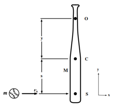
When an impulsive force P strikes a bat of mass M at a distance s from the center of mass, then both the linear momentum of the center of mass, and angular momenta about the center of mass, of the bat are changed. Assume that the ball strikes the bat with an impulsive force \( P = \Delta p ^{ball} \) perpendicular to the symmetry axis of the bat at the strike point S which is a distance s from the center of mass of the bat. The translational impulse given to the bat equals the change in linear momentum of the ball as given by equation 2.136 coupled with the conservation of linear momentum

\[ \nonumber \mathbf{P} = \Delta\mathbf{p}_{cm}^{bat} = M \Delta\mathbf{v}_{cm}^{bat} \]

Similarly equation 2.142 gives that the angular impulse T equals the change in angular momentum about the center of mass to be

\[ \mathbf{T} = s \times \mathbf{P} = \Delta \mathbf{L} = I_{cm} \Delta \omega_{cm} \]

The above equations give that

\[ \nonumber \begin{align*} \Delta \mathbf{v}_{cm}^{bat} & = &  \frac{\mathbf{P}}{M}  \\ \Delta \mathbf{\omega} & = & \frac{\mathbf{s} \times \mathbf{P}}{\mathbf{I}_{cm}} \end{align*} \]

Assume that the bat was stationary prior to the strike, then after the strike the net translational velocity of a point O along the body-fixed symmetry axis of the bat at a distance y from the center of mass, is given by

\[ \nonumber \mathbf{v} (y) = \Delta \mathbf{v}_{cm} + \Delta \omega_{cm} \times \mathbf{y} = \frac{\mathbf{P}}{M} + \frac{1}{I_cm}( ( \mathbf{s} \times \mathbf{P} ) \times y ) = \frac{\mathbf{P}}{M} + \frac{1}{I_{cm}} [ ( \mathbf{s \cdot y ) P - (s \cdot P ) y }] \]

It is assumed that P and s are perpendicular and thus \( \mathbf{s \times P } = 0 \) which simplifies the above equation to

\[ \nonumber \mathbf{v} (y) = \Delta \mathbf{v}_{cm} + \Delta \mathbf{\omega}_{cm} \times \mathbf{y} = \frac{\mathbf{P}}{M} \bigg ( 1 + \frac{M ( \mathbf{s \cdot y} )}{I_{cm}} \bigg ) \]

Note that the translational velocity of the location O, along the bat symmetry axis at a distance y from the center of mass, is zero if the bracket equals zero, that is, if

\[ \nonumber \mathbf{s \cdot y} = - \frac{I_{cm}}{M} = - k^2_{cm} \]

where \( k_{cm} \) is called the radius of gyration of the body about the center of mass. Note that when the scalar product \( s \cdot y = - \frac{I_{cm}}{M} \) then there will be no translational motion at the point O. This point on the y axis lies on the opposite side of the center of mass from the strike point S, and is called the center of percussion corresponding to the impulse at the point S. The center of percussion often is referred to as the "sweet spot" for an object corresponding to the impulse at the point S. For a baseball bat the batter holds the bat at the center of percussion so that they do not feel an impulse in their hands when the ball is struck at the point S. This principle is used extensively to design bats for all sports involving striking a ball with a bat, such as, cricket, squash, tennis, etc. as well as weapons such of swords and axes used to decapitate opponents.

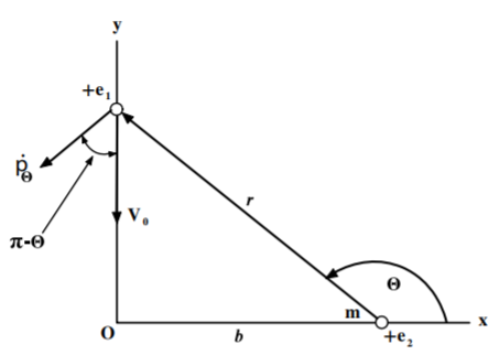
2.15 Example: Energy transfer in charged-particle scattering

Consider a particle of charge \( + e_1 \) moving with very high velocity \( v_0 \) along a straight line that passes a distance b from another charge \( + e_2 \) and mass m. Find the energy Q transferred to the mass m during the encounter assuming the force is given by Coulomb’s law. Since the charged particle \( e_1 \) moves at very high speed it is assumed that charge 2 does not change position during the encounter. Assume that charge 1 moves along the −y axis through the origin while charge 2 is located on the x axis at x = b. Let us consider the impulse given to charge 2 during the encounter. By symmetry the y component must cancel while the x component is given by

\[ \nonumber dp_x = F_xdt = -\frac{\epsilon_1\epsilon_2}{4 \pi \varepsilon_0r^2} \cos \theta dt = -\frac{\epsilon_1\epsilon_2}{4 \pi \varepsilon_0r^2} \cos \theta \frac{dt}{d \theta}d\theta \]

But

\[ \nonumber r\dot{\theta} = - v_0 \cos \theta \]

where

\[\nonumber \frac{b}{r} = \cos ( \pi - \theta ) = -\cos \theta \]

Thus

\[\nonumber dp_x = -\frac{\epsilon_1\epsilon_2}{4 \pi \varepsilon_0 b v_0} \cos \theta d\theta \]

Integrate from \( \frac{\pi}{2} < \theta < \frac{3 \pi}{2} \) gives that the total momentum imparted to \( \epsilon_2 \) is

\[\nonumber p_x = -\frac{\epsilon_1 \epsilon_2}{4 \pi \varepsilon_0 b v_0} \int_{\frac{\pi}{2}}^{\frac{3 \pi}{2}} \cos \theta d \theta = \frac{\epsilon_1 \epsilon_2}{2 \pi \epsilon_0 b v_0} \]

Thus the recoil energy of charge 2 is given by

\[\nonumber E_2 = \frac{p_x ^2}{2m} = \frac{1}{2m} \bigg ( \frac{\epsilon_1\epsilon_2}{2 \pi \epsilon_0 b v_0} \bigg ) ^2 \]