
6.3: The Schwarzschild Metric (Part 2)
- Page ID
- 10454

Geodetic Effect
As promised in section 5.5, we now calculate the geodetic effect on Gravity Probe B, including all the niggling factors of 3 and \(\pi\). To make the physics clear, we approach the actual calculation through a series of warmups.
Flat Space
As a first warmup, consider two spatial dimensions, represented by Euclidean polar coordinates (r, \(\phi\)). Parallel-transport of a gyroscope’s angular momentum around a circle of constant r gives
\[\begin{split} \nabla_{\phi} L^{\phi} &= 0 \\ \nabla_{\phi} L^{r} &= 0 \ldotp \end{split}\]
Computing the covariant derivatives, we have
\[\begin{split} 0 &= \partial_{\phi} L^{\phi} + \Gamma^{\phi}_{\phi r} L^{r} \\ 0 &= \partial_{\phi} L^{r} + \Gamma^{r}_{\phi \phi} L^{\phi} \ldotp \end{split}\]
The Christoffel symbols are \(\Gamma^{\phi}_{\phi r} = \frac{1}{r}\) and \(\Gamma^{r}_{\phi \phi}\) = −r. This is all made to look needlessly complicated because L\(\phi\) and Lr are expressed in different units. Essentially the vector is staying the same, but we’re expressing it in terms of basis vectors in the r and \(\phi\) directions that are rotating. To see this more transparently, let r = 1, and write P for L\(\phi\) and Q for Lr, so that
\[\begin{split} P' &= -Q \\ Q' &= P, \end{split}\]
which have solutions such as P = sin \(\phi\), Q = cos \(\phi\). For each orbit (2π\(\pi\)change in \(\phi\)), the basis vectors rotate by 2\(\phi\), so the angular momentum vector once again has the same components. In other words, it hasn’t really changed at all.
Spatial Curvature Only
The flat-space calculation above differs in two ways from the actual result for an orbiting gyroscope: (1) it uses a flat spatial geometry, and (2) it is purely spatial. The purely spatial nature of the calculation is manifested in the fact that there is nothing in the result relating to how quickly we’ve moved the vector around the circle. We know that if we whip a gyroscope around in a circle on the end of a rope, there will be a Thomas precession (section 2.5), which depends on the speed.
As our next warmup, let’s curve the spatial geometry, but continue to omit the time dimension. Using the Schwarzschild metric, we replace the flat-space Christoffel symbol \(\Gamma^{r}_{\phi \phi}\) = −r with −r+2m. The differential equations for the components of the L vector, again evaluated at r = 1 for convenience, are now
\[\begin{split} P' &= -Q \\ Q' &= (1 - \epsilon) P, \end{split}\]
where \(\epsilon\) = 2m. The solutions rotate with frequency \(\omega' = \sqrt{1 − \epsilon}\). The result is that when the basis vectors rotate by 2\(\pi\), the components no longer return to their original values; they lag by a factor of \(\sqrt{1 − \epsilon}\) ≈ 1 − m. Putting the factors of r back in, this is 1 − \(\frac{m}{r}\). The deviation from unity shows that after one full revolution, the L vector no longer has quite the same components expressed in terms of the (r, \(\phi\)) basis vectors.
To understand the sign of the effect, let’s imagine a counterclockwise rotation. The (r, \(\phi\)) rotate counterclockwise, so relative to them, the L vector rotates clockwise. After one revolution, it has not rotated clockwise by a full 2\(\pi\), so its orientation is now slightly counterclockwise compared to what it was. Thus the contribution to the geodetic effect arising from spatial curvature is in the same direction as the orbit.
Comparing with the actual results from Gravity Probe B, we see that the direction of the effect is correct. The magnitude, however, is off. The precession accumulated over n periods is \(\frac{2 \pi nm}{r}\), or, in SI units, \(\frac{2 \pi nGm}{c^{2} r}\). Using the data from section 2.5, we find \(\Delta \theta\) = 2 × 10⁻⁵ radians, which is too small compared to the data shown in Figure 5.5.2.
2+1 Dimensions
To reproduce the experimental results correctly, we need to include the time dimension. The angular momentum vector now has components (L\(\phi\),Lr,Lt). The physical interpretation of the Lt component is obscure at this point; we’ll return to this question later.
Writing down the total derivatives of the three components, and notating \(\frac{dt}{d \phi}\) as \(\omega^{−1}\), we have
\[\frac{dL^{\phi}}{d \phi} = \partial_{\phi} L^{\phi} + \omega^{-1} \partial_{t} L^{\phi}\]
\[\frac{dL^{r}}{d \phi} = \partial_{\phi} L^{r} + \omega^{-1} \partial_{t} L^{r}\]
\[\frac{dL^{t}}{d \phi} = \partial_{\phi} L^{t} + \omega^{-1} \partial_{t} L^{t}\]
Setting the covariant derivatives equal to zero gives
\[\begin{split} 0 &= \partial_{\phi} L^{\phi} + \Gamma^{\phi}_{\phi r} L^{r} \\ 0 &= \partial_{\phi} L^{r} + \Gamma^{r}_{\phi \phi} L^{\phi} \\ 0 &= \partial_{t} L^{r} + \Gamma^{r}_{tt} L^{t} \\ 0 &= \partial_{t} L^{t} + \Gamma^{t}_{tr} L^{r} \ldotp \end{split}\]
Exercise \(\PageIndex{4}\)
Self-check: There are not just four but six covariant derivatives that could in principle have occurred, and in these six covariant derivatives we could have had a total of 18 Christoffel symbols. Of these 18, only four are nonvanishing. Explain based on symmetry arguments why the following Christoffel symbols must vanish: \(\Gamma^{\phi}_{\phi t}, \Gamma^{t}_{tt}\).
Putting all this together in matrix form, we have L' = ML, where
\[M = \begin{pmatrix} 0 & -1 & 0 \\ 1 - \epsilon & 0 & - \frac{\epsilon (1 - \epsilon)}{2 \omega} \\ 0 & - \frac{\epsilon}{2 \omega (1 - \epsilon)} & 0 \end{pmatrix} \ldotp\]
The solutions of this differential equation oscillate like ei\(\Omega\)t, where i\(\Omega\) is an eigenvalue of the matrix.
Exercise \(\PageIndex{5}\)
Self-check: The frequency in the purely spatial calculation was found by inspection. Verify the result by applying the eigenvalue technique to the relevant 2 × 2 submatrix.
To lowest order, we can use the Newtonian relation \(\omega^{2} r = \frac{Gm}{r}\) and neglect terms of order \(\epsilon^{2}\), so that the two new off-diagonal matrix elements are both approximated as \(\sqrt{\frac{\epsilon}{2}}\). The three resulting eigenfrequencies are zero and \(\Omega\) = ±[1 − \(\frac{3}{2}\))m/r].
The presence of the mysterious zero-frequency solution can now be understood by recalling the earlier mystery of the physical interpretation of the angular momentum’s Lt component. Our results come from calculating parallel transport, and parallel transport is a purely geometric process, so it gives the same result regardless of the physical nature of the four-vector. Suppose that we had instead chosen the velocity four-vector as our guinea pig. The definition of a geodesic is that it parallel-transports its own tangent vector, so the velocity vector has to stay constant. If we inspect the eigenvector corresponding to the zero-frequency eigenfrequency, we find a timelike vector that is parallel to the velocity four-vector. In our 2+1-dimensional space, the other two eigenvectors, which are spacelike, span the subspace of spacelike vectors, which are the ones that can physically be realized as the angular momentum of a gyroscope. These two eigenvectors, which vary as e±i\(\Omega\), can be superposed to make real-valued spacelike solutions that match the initial conditions, and these lag the rotation of the basis vectors by \(\Delta \Omega\) = \(\frac{3}{2}\)mr. This is greater than the purely spatial result by a factor of \(\frac{3}{2}\). The resulting precession angle, over n orbits of Gravity Probe B, is \(\frac{3 \pi nGm}{c^{2} r}\) = 3 × 10⁻⁵ radians, in excellent agreement with experiment.
One will see apparently contradictory statements in the literature about whether Thomas precession occurs for a satellite: “The Thomas precession comes into play for a gyroscope on the surface of the Earth . . . , but not for a gyroscope in a freely moving satellite.”6 But: “The total effect, geometrical and Thomas, gives the well-known Fokker-de Sitter precession of \(\frac{3 \pi m}{r}\), in the same sense as the orbit.”7 The second statement arises from subtracting the purely spatial result from the 2+1-dimensional result, and noting that the absolute value of this difference is the same as the Thomas precession that would have been obtained if the gyroscope had been whirled at the end of a rope. In my opinion this is an unnatural way of looking at the physics, for two reasons. (1) The signs don’t match, so one is forced to say that the Thomas precession has a different sign depending on whether the rotation is the result of gravitational or nongravitational forces. (2) Referring to observation, it is clearly artificial to treat the spatial curvature and Thomas effects separately, since neither one can be disentangled from the other by varying the quantities n, m, and r. For more discussion, see tinyurl.com/me3qf8o.
Orbits
The main event of Newton’s Principia Mathematica is his proof of Kepler’s laws. Similarly, Einstein’s first important application in general relativity, which he began before he even had the exact form of the Schwarzschild metric in hand, was to find the non-Newtonian behavior of the planet Mercury. The planets deviate from Keplerian behavior for a variety of Newtonian reasons, and in particular there is a long list of reasons why the major axis of a planet’s elliptical orbit is expected to gradually rotate. When all of these were taken into account, however, there was a remaining discrepancy of about 40 seconds of arc per century, or 6.6 × 10⁻⁷ radians per orbit. The direction of the effect was in the forward direction, in the sense that if we view Mercury’s orbit from above the ecliptic, so that it orbits in the counterclockwise direction, then the gradual rotation of the major axis is also counterclockwise.
As a very rough hand-wavy explanation for this effect, consider the spatial part of the curvature of the spacetime surrounding the sun. This spatial curvature is positive, so a circle’s circumference is less than 2\(\pi\) times its radius. We could imagine that this would cause Mercury to get back to a previously visited angular position before it has had time to complete its Newtonian cycle of radial motion. Arguments such as this one, however, should not be taken too seriously. A mathematical analysis is required.
Based on the examples in section 5.5, we expect that the effect will be of order \(\frac{m}{r}\), where m is the mass of the sun and r is the radius of Mercury’s orbit. This works out to be 2.5 × 10⁻⁸, which is smaller than the observed precession by a factor of about 26.
Conserved Quantities
If Einstein had had a computer on his desk, he probably would simply have integrated the motion numerically using the geodesic equation. But it is possible to simplify the problem enough to attack it with pencil and paper, if we can find the relevant conserved quantities of the motion. Nonrelativistically, these are energy and angular momentum.
Consider a rock falling directly toward the sun. The Schwarzschild metric is of the special form
\[ds^{2} = h(r) dt^{2} - k(r) dr^{2} - \ldots\]
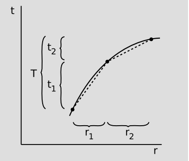
The rock’s trajectory is a geodesic, so it extremizes the proper time s between any two events fixed in spacetime, just as a piece of string stretched across a curved surface extremizes its length. Let the rock pass through distance r1 in coordinate time t1, and then through r2 in t2. (These should really be notated as \(\Delta\)r1, . . . or dr1, . . . , but we avoid the \(\Delta\)’s or d’s for convenience.) Approximating the geodesic using two line segments, the proper time is
\[\begin{split} s &= s_{1} + s_{2} \\ &= \sqrt{h_{1} t_{1}^{2} - k_{1} r^{2}_{1}} + \sqrt{h_{2} t_{2}^{2} - k_{2} r^{2}_{2}} \\ &= \sqrt{h_{1} t_{1}^{2} - k_{1} r^{2}_{1}} + \sqrt{h_{2} (T - t_{1})^{2} - k_{2} r^{2}_{2}}, \end{split}\]
where T = t1 + t2 is fixed. If this is to be extremized with respect to t1, then \(\frac{ds}{dt_{1}}\) = 0, which leads to
\[0 = \frac{h_{1} t_{1}}{s_{1}} - \frac{h_{2} t_{2}}{s_{2}},\]
which means that
\[h \frac{dt}{ds} = g_{tt} \frac{dx^{t}}{ds} = \frac{dx_{t}}{ds}\]
is a constant of the motion. Except for an irrelevant factor of m, this is the same as pt, the timelike component of the covariant momentum vector. We’ve already seen that in special relativity, the timelike component of the momentum four-vector is interpreted as the mass-energy E, and the quantity pt has a similar interpretation here. Note that no special assumption was made about the form of the functions h and k. In addition, it turns out that the assumption of purely radial motion was unnecessary. All that really mattered was that h and k were independent of t. Therefore we will have a similar conserved quantity p\(\mu\) any time the metric’s components, expressed in a particular coordinate system, are independent of x\(\mu\). (This is generalized in section 7.1.) In particular, the Schwarzschild metric’s components are independent of \(\phi\) as well as t, so we have a second conserved quantity p\(\phi\), which is interpreted as angular momentum.
Writing these two quantities out explicitly in terms of the contravariant coordinates, in the case of the Schwarzschild spacetime, we have
\[E = \left(1 - \dfrac{2m}{r}\right) \frac{dt}{ds}\]
and
\[L = r^{2} \frac{d \phi}{ds}\]
for the conserved energy per unit mass and angular momentum per unit mass.
In interpreting the energy per unit mass E, it is important to understand that in the general-relativistic context, there is no useful way of separating the rest mass, kinetic energy, and potential energy into separate terms, as we could in Newtonian mechanics. E includes contributions from all of these, and turns out to be less than the contribution due to the rest mass (i.e., less than 1) for a planet orbiting the sun. It turns out that E can be interpreted as a measure of the additional gravitational mass that the solar system possesses as measured by a distant observer, due to the presence of the planet. It then makes sense that E is conserved; by analogy with Newtonian mechanics, we would expect that any gravitational effects that depended on the detailed arrangement of the masses within the solar system would decrease as \(\frac{1}{r^{4}}\), becoming negligible at large distances and leaving a constant field varying as \(\frac{1}{r^{2}}\).
One way of seeing that it doesn’t make sense to split E into parts is that although the equation given above for E involves a specific set of coordinates, E can actually be expressed as a Lorentz-invariant scalar (see section 7.1). This property makes E especially interesting and useful (and different from the energy in Newtonian mechanics, which is conserved but not frame-independent). On the other hand, the kinetic and potential energies depend on the velocity and position. These are completely dependent on the coordinate system, and there is nothing physically special about the coordinate system we’ve used here. Suppose a particle is falling directly toward the earth, and an astronaut in a space-suit is free-falling along with it and monitoring its progress. The astronaut judges the particle’s kinetic energy to be zero, but other observers say it’s nonzero, so it’s clearly not a Lorentz scalar. And suppose the astronaut insists on defining a potential energy to go along with this kinetic energy. The potential energy must be decreasing, since the particle is getting closer to the earth, but then there is no way that the sum of the kinetic and potential energies could be constant.
Perihelion Advance
For convenience, let the mass of the orbiting rock be 1, while m stands for the mass of the gravitating body.
The unit mass of the rock is a third conserved quantity, and since the magnitude of the momentum vector equals the square of the mass, we have for an orbit in the plane \(\theta = \frac{\pi}{2}\),
\[\begin{split} 1 &= g^{tt} p_{t}^{2} - g^{rr} p^{2}_{r} - g^{\phi \phi} p_{\phi}^{2} \\ &= g^{tt} p_{t}^{2} g_{rr} (p^{r})^{2} - g^{\phi \phi} p_{\phi}^{2} \\ &= \frac{1}{1 - \frac{2m}{r}} E^{2} - \frac{1}{1 - \frac{2m}{r}} \left(\dfrac{dr}{ds}\right)^{2} - \frac{1}{r^{2}} L^{2} \ldotp \end{split}\]
Rearranging terms and writing \(\dot{r}\) for \(\frac{dr}{ds}\), this becomes
\[\dot{r}^{2} = E^{2} - \left(1 - \dfrac{2m}{r}\right) \left(d\frac{1 + L^{2}}{r^{2}}\right)\]
or
\[\dot{r}^{2} = E^{2} - U^{2}\]
where
\[U^{2} = \left(1 - \frac{2m}{r}\right) \left(1 + \dfrac{L^{2}}{r^{2}}\right) \ldotp\]
There is a varied and strange family of orbits in the Schwarzschild field, including bizarre knife-edge trajectories that take several nearly circular turns before suddenly flying off. We turn our attention instead to the case of an orbit such as Mercury’s which is nearly Newtonian and nearly circular.
Nonrelativistically, a circular orbit has radius \(r = \frac{L^{2}}{m}\) and period \(T = \frac{2 \pi L^{3}}{m^{2}}\).
Relativistically, a circular orbit occurs when there is only one turning point at which \(\dot{r}\) = 0. This requires that E2 equal the minimum value of U2, which occurs at
\[\begin{split} r &= \frac{L^{2}}{2m} \left(1 + \sqrt{1 - \dfrac{12m^{2}}{L^{2}}}\right) \\ &\approx \frac{L^{2}}{m} (1 - \epsilon), \end{split}\]
where \(\epsilon = 3(\frac{m}{L})^{2}\). A planet in a nearly circular orbit oscillates between perihelion and aphelion with a period that depends on the curvature of U2 at its minimum. We have
\[\begin{split} k &= \frac{d^{2} (U^{2})}{dr^{2}} \\ &= \frac{d^{2}}{dr^{2}} \left(1 - \dfrac{2m}{r} + \dfrac{L^{2}}{r^{2}} - \dfrac{2mL^{2}}{r^{3}}\right) \\ &= - \frac{4m}{r^{3}} + \frac{6L^{2}}{r^{4}} - \frac{24 mL^{2}}{r^{5}} \\ &= 2L^{-6} m^{4} (1 + 2 \epsilon) \end{split}\]
The period of the oscillations is
\[\begin{split} \Delta s_{osc} &= 2 \pi \sqrt{\frac{2}{k}} \\ &= 2 \pi L^{3} m^{-2} (1 - 2 \epsilon) \ldotp \end{split}\]
The period of the azimuthal motion is
\[\begin{split} \Delta s_{az} &= \frac{2 \pi r^{2}}{L} \\ &= 2 \pi L^{3} m^{-2} (1 - 2 \epsilon) \ldotp \end{split}\]
The periods are slightly mismatched because of the relativistic correction terms. The period of the radial oscillations is longer, so that, as expected, the perihelion shift is in the forward direction. The mismatch is \(\epsilon \Delta\)s, and because of it each orbit rotates the major axis by an angle \(2 \pi \epsilon = 6 \pi (\frac{m}{L})^{2} = \frac{6 \pi m}{r}\). Plugging in the data for Mercury, we obtain 5.8 × 10⁻⁷ radians per orbit, which agrees with the observed value to within about 10%. Eliminating some of the approximations we’ve made brings the results in agreement to within the experimental error bars, and Einstein recalled that when the calculation came out right, “for a few days, I was beside myself with joyous excitement.”
Further attempts were made to improve on the precision of this historically crucial test of general relativity. Radar now gives the most precise orbital data for Mercury. At the level of about one part per thousand, however, an effect creeps in due to the oblateness of the sun, which is difficult to measure precisely.
In 1974, astronomers J.H. Taylor and R.A. Hulse of Princeton, working at the Arecibo radio telescope, discovered a binary star system whose members are both neutron stars. The detection of the system was made possible because one of the neutron stars is a pulsar: a neutron star that emits a strong radio pulse in the direction of the earth once per rotational period. The orbit is highly elliptical, and the minimum separation between the two stars is very small, about the same as the radius of our sun. Both because the r is small and because the period is short (about 8 hours), the rate of perihelion advance per unit time is very large, about 4.2 degrees per year. The system has been compared in great detail with the predictions of general relativity,8 giving extremely good agreement, and as a result astronomers have been confident enough to reason in the opposite direction and infer properties of the system, such as its total mass, from the general-relativistic analysis. The system’s orbit is decaying due to the radiation of energy in the form of gravitational waves, which are predicted to exist by relativity.
Deflection of Light
As discussed in section 5.5, one of the first tests of general relativity was Eddington’s measurement of the deflection of rays of light by the sun’s gravitational field. The deflection measured by Eddington was 1.6 seconds of arc. For a light ray that grazes the sun’s surface, the only physically relevant parameters are the sun’s mass m and radius r. Since the deflection is unitless, it can only depend on \(\frac{m}{r}\), the unitless ratio of the sun’s mass to its radius. Expressed in SI units, this is \(\frac{Gm}{c^{2} r}\), which comes out to be about 10−6. Roughly speaking, then, we expect the order of magnitude of the effect to be about this big, and indeed 10−6 radians comes out to be in the same ball-park as a second of arc. We get a similar estimate in Newtonian physics by treating a photon as a (massive) particle moving at speed c.
It is possible to calculate a precise value for the deflection using methods very much like those used to determine the perihelion advance from earlier. However, some of the details would have to be changed. For example, it is no longer possible to parametrize the trajectory using the proper time s, since a light ray has ds = 0; we must use an affine parameter. Let us instead use this an an example of the numerical technique for solving the geodesic equation, first demonstrated in section 5.9. Modifying our earlier program, we have the following:
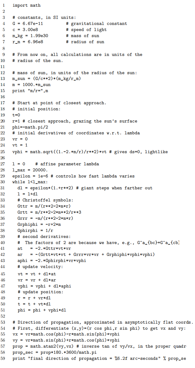
At line 14, we take the mass to be 1000 times greater than the mass of the sun. This helps to make the deflection easier to calculate accurately without running into problems with rounding errors. Lines 17-25 set up the initial conditions to be at the point of closest approach, as the photon is grazing the sun. This is easier to set up than initial conditions in which the photon approaches from far away. Because of this, the deflection angle calculated by the program is cut in half. Combining the factors of 1000 and one half, the final result from the program is to be interpreted as 500 times the actual deflection angle.
The result is that the deflection angle is predicted to be 870 seconds of arc. As a check, we can run the program again with m = 0; the result is a deflection of −8 seconds, which is a measure of the accumulated error due to rounding and the finite increment used for \(\lambda\).
Dividing by 500, we find that the predicted deflection angle is 1.74 seconds, which, expressed in radians, is exactly \(\frac{4Gm}{c^{2} r}\). The unitless factor of 4 is in fact the correct result in the case of small deflections, i.e., for \(\frac{m}{r}\) << 1.
Although the numerical technique has the disadvantage that it doesn’t let us directly prove a nice formula, it has some advantages as well. For one thing, we can use it to investigate cases for which the approximation \(\frac{m}{r}\) << 1 fails. For \(\frac{m}{r}\) = 0.3, the numerical technique gives a deflection of 222 degrees, whereas the weak-field approximation \(\frac{4Gm}{c^{2} r}\) gives only 69 degrees. What is happening here is that we’re getting closer and closer to the event horizon of a black hole. Black holes are the topic of section 6.3, but it should be intuitively reasonable that something wildly nonlinear has to happen as we get close to the point where the light wouldn’t even be able to escape.
The precision of Eddington’s original test was only about ± 30%, and has never been improved on significantly with visible-light astronomy. A better technique is radio astronomy, which allows measurements to be carried out without waiting for an eclipse. One merely has to wait for the sun to pass in front of a strong, compact radio source such as a quasar. These techniques have now verified the deflection of light predicted by general relativity to a relative precision of about 10−5.9
References
6 Misner, Thorne, and Wheeler, Gravitation, p. 1118
7 Rindler, Essential Relativity, 1969, p. 141
9 For a review article on this topic, see Clifford Will, “The Confrontation between General Relativity and Experiment,” relativity.livingreviews.org/...es/lrr-2006-3/.