5.10: From Metric to Curvature

Finding the Christoffel Symbol from the Metric

We’ve already found the Christoffel symbol in terms of the metric in one dimension. Expressing it in tensor notation, we have

\[\Gamma^{d}_{ba} = \frac{1}{2} g^{cd} (\partial_{?} g_{??}),\]

where inversion of the one-component matrix G has been replaced by matrix inversion, and, more importantly, the question marks indicate that there would be more than one way to place the subscripts so that the result would be a grammatical tensor equation. The most general form for the Christoffel symbol would be

\[\Gamma^{b}_{ac} = \frac{1}{2} g^{db} (L \partial_{c} g_{ab} + M \partial_{a} g_{cb} + N \partial_{b} g_{ca}),\]

where \(L\), \(M\), and \(N\) are constants. Consistency with the onedimensional expression requires

\[L + M + N = 1\]

and vanishing torsion gives \(L = M\). The \(L\) and \(M\) terms have a different physical significance than the \(N\) term.

Suppose an observer uses coordinates such that all objects are described as lengthening over time, and the change of scale accumulated over one day is a factor of k > 1. This is described by the derivative \(\partial_{t} g_{xx}\) < 1, which affects the \(M\) term. Since the metric is used to calculate squared distances, the g_xx matrix element scales down by \(\frac{1}{\sqrt{k}}\). To compensate for \(\partial_{t} v^{x} < 0\), so we need to add a positive correction term, \(M > 0\), to the covariant derivative. When the same observer measures the rate of change of a vector \(v^t\) with respect to space, the rate of change comes out to be too small, because the variable she differentiates with respect to is too big. This requires \(N < 0\), and the correction is of the same size as th\(M\) correction, so \(|M| = |N|\). We find \(L = M = −N = 1\).

Exercise \(\PageIndex{1}\)

Does the above argument depend on the use of space for one coordinate and time for the other?

The resulting general expression for the Christoffel symbol in terms of the metric is

\[\Gamma^{c}_{ab} = \frac{1}{2} g^{cd} (\partial_{a} g_{bd} + \partial_{b} g_{ad} - \partial_{d} g_{ab}) \ldotp\]

One can readily go back and check that this gives

\[\nabla_{c} g_{ab} = 0. \label{eq10}\]

Confirming Equation \ref{eq10} is a bit tedious. For that matter, tensor calculations in general can be infamously time-consuming and error-prone. Any reasonable person living in the 21st century will therefore resort to a computer algebra system. The most widely used computer algebra system is Mathematica, but it’s expensive and proprietary, and it doesn’t have extensive built-in facilities for handling tensors. It turns out that there is quite a bit of free and open-source tensor software, and it falls into two classes: coordinate-based and coordinate-independent. The best open-source coordinate-independent facility available appears to be Cadabra, and in fact the verification of \(\nabla_{c} g_{ab}\) = 0 is the first example given in the Leo Brewin’s handy guide to applications of Cadabra to general relativity.¹³

Exercise \(\PageIndex{2}\)

In the case of 1 dimension, show that this reduces to the earlier result of \(−(\frac{1}{2}) \frac{dG}{dX}\).

Since \(\Gamma\) is not a tensor, it is not obvious that the covariant derivative, which is constructed from it, is a tensor. But if it isn’t obvious, neither is it surprising – the goal of the above derivation was to get results that would be coordinate-independent.

Example 10: Christoffel symbols on the globe, quantitatively

In example 9, we inferred the following properties for the Christoffel symbol \(\Gamma^{\theta}_{\phi \phi}\) on a sphere of radius R: \(\Gamma^{\theta}_{\phi \phi}\) is independent of \(\phi\) and R, \(\Gamma^{\theta}_{\phi \phi}\) < 0 in the northern hemisphere (colatitude θ less than π/2), \(\Gamma^{\theta}_{\phi \phi}\) = 0 on the equator, and \(\Gamma^{\theta}_{\phi \phi}\) > 0 in the southern hemisphere.

The metric on a sphere is

\[ds^2 = R^2 d\theta^{2} + R^2 \sin^2 \theta d\phi^{2}.\]

The only nonvanishing term in the expression for \(\Gamma^{\theta}_{\phi \phi}\) is the one involving \(\partial_{\theta} g_{\phi \phi} = 2R^{2} \sin \theta \cos \theta\). The result is

\[\Gamma^{\theta}_{\phi \phi} = − \sin \theta \cos \theta\]

which can be verified to have the properties claimed above.

Numerical Solution of the Geodesic Equation

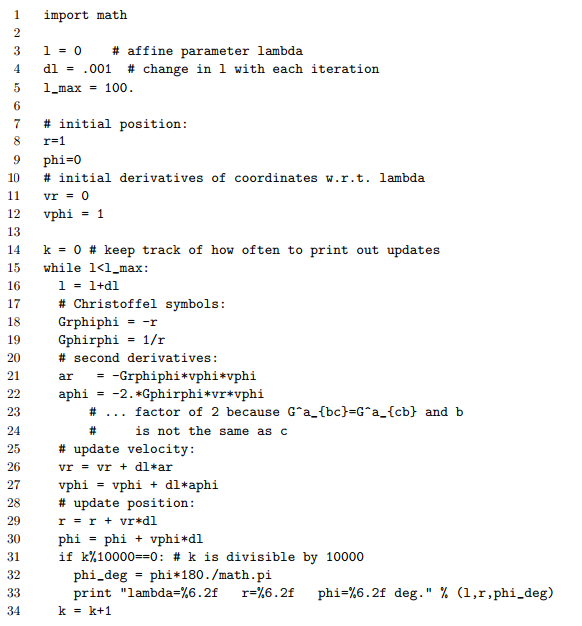
In Section 5.7, I gave an algorithm that demonstrated the uniqueness of the solutions to the geodesic equation. This algorithm can also be used to find geodesics in cases where the metric is known. The following program, written in the computer language Python, carries out a very simple calculation of this kind, in a case where we know what the answer should be; even without any previous familiarity with Python, it shouldn’t be difficult to see the correspondence between the abstract algorithm presented in Section 5.7 and its concrete realization below. For polar coordinates in a Euclidean plane, one can compute \(\Gamma^{r}_{\phi \phi}\) = −r and \(\Gamma^{\phi}_{r \phi} = \frac{1}{r}\) (problem 2). Here we compute the geodesic that starts out tangent to the unit circle at \(\phi=0\).

It is not necessary to worry about all the technical details of the language (e.g., line 1, which makes available such conveniences as math.pi for \(\pi\)). Comments are set off by pound signs. Lines 16-34 are indented because they are all to be executed repeatedly, until it is no longer true that \(\lambda < \lambda_{max}\) (line 15).

Exercise \(\PageIndex{3}\)

By inspecting lines 18-22, find the signs of \(\ddot{r}\) and \(\ddot{\phi}\) at \(\lambda\) = 0. Convince yourself that these signs are what we expect geometrically.

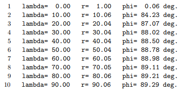
The output is as follows:

We can see that \(\phi\) → 90 deg. as \(\lambda \rightarrow \infty\), which makes sense, because the geodesic is a straight line parallel to the y axis. A less trivial use of the technique is demonstrated in Section 6.2, where we calculate the deflection of light rays in a gravitational field, one of the classic observational tests of general relativity.

The Riemann Tensor in Terms of the Christoffel Symbols

The covariant derivative of a vector can be interpreted as the rate of change of a vector in a certain direction, relative to the result of parallel-transporting the original vector in the same direction. We can therefore see that the definition of the Riemann curvature tensor in Section 5.4 is a measure of the failure of covariant derivatives to commute:

\[(\nabla_{a} \nabla_{b} - \nabla_{b} \nabla_{a}) A^{c} = A^{d} R^{c}_{dab}\]

A tedious calculation now gives \(R\) in terms of the \(\Gamma\)s:

\[R^{a}_{bcd} = \partial_{c} \Gamma^{a}_{db} - \partial_{d} \Gamma^{a}_{cb} + \Gamma^{a}_{ce} \Gamma^{e}_{db} - \Gamma^{a}_{de} \Gamma^{e}_{cb}\]

This is given as another example later in Brewin’s manual for applying Cadabra to general relativity.¹⁴ (Brewin writes the upper index in the second slot of R.)

Some General Ideas about Gauge

Let’s step back now for a moment and try to gain some physical insight by looking at the features that the electromagnetic and relativistic gauge transformations have in common. We have the following analogies:

	electromagnetism	differential geometry
global symmetry	A constant phase shift \(\alpha\) has no observable effects.	Adding a constant onto a coordinate has no observable effects.
local symmetry	A phase shift \(\alpha\) that varies from point to point has no observable effects.	An arbitrary coordinate transformation has no observable effects.
The gauge is described by . . .	\(\alpha\)	\(g_{\mu \nu}\)
. . . and differentiation of this gives the gauge field. . .	Ab	\(\Gamma^{c}_{ab}\)
A second differentiation gives the directly observable field(s) . . .	E and B	\(R^c_{dab}\)

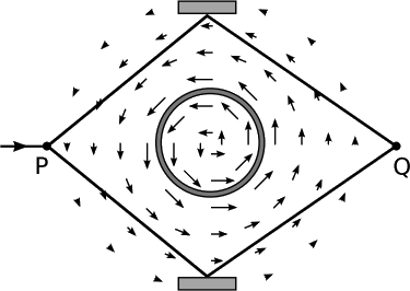
The interesting thing here is that the directly observable fields do not carry all of the necessary information, but the gauge fields are not directly observable. In electromagnetism, we can see this from the Aharonov-Bohm effect, shown in Figure \(\PageIndex{1}\).¹⁵ The solenoid has B = 0 externally, and the electron beams only ever move through the external region, so they never experience any magnetic field. Experiments show, however, that turning the solenoid on and off does change the interference between the two beams. This is because the vector potential does not vanish outside the solenoid, and as we’ve seen in section 4.2, the phase of the beams varies according to the path integral of the A_b. We are therefore left with an uncomfortable, but unavoidable, situation. The concept of a field is supposed to eliminate the need for instantaneous action at a distance, which is forbidden by relativity; that is, (1) we want our fields to have only local effects. On the other hand, (2) we would like our fields to be directly observable quantities. We cannot have both 1 and 2. The gauge field satisfies 1 but not 2, and the electromagnetic fields give 2 but not 1.

Figure \(\PageIndex{1}\): The Aharonov-Bohm effect. An electron enters a beam splitter at P, and is sent out in two different directions. The two parts of the wave are reflected so that they reunite at Q. The arrows represent the vector potential A. The observable magnetic field B is zero everywhere outside the solenoid, and yet the interference observed at Q depends on whether the field is turned on. See section 4.2 for further discussion of the A and B fields of a solenoid.

Note

We describe the effect here in terms of an idealized, impractical experiment. For the actual empirical status of the Aharonov-Bohm effect, see Batelaan and Tonomura, Physics Today 62 (2009) 38.

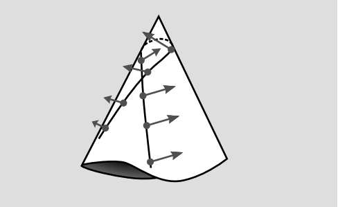
Figure 5.9.2 shows an analog of the Aharonov-Bohm experiment in differential geometry. Everywhere but at the tip, the cone has zero curvature, as we can see by cutting it and laying it out flat. But even an observer who never visits the tightly curved region at the tip can detect its existence, because parallel-transporting a vector around a closed loop can change the vector’s direction, provided that the loop surrounds the tip.

Figure \(\PageIndex{2}\) - The cone has zero intrinsic curvature everywhere except at its tip. An observer who never visits the tip can nevertheless detect its existence, because parallel transport around a path that encloses the tip causes a vector to change its direction.

In the electromagnetic example, integrating A around a closed loop reveals, via Stokes’ theorem, the existence of a magnetic flux through the loop, even though the magnetic field is zero at every location where A has to be sampled. In the relativistic example, integrating \(\Gamma\) around a closed loop shows that there is curvature inside the loop, even though the curvature is zero at all the places where \(\Gamma\) has to be sampled.

The fact that \(\Gamma\) is a gauge field, and therefore not locally observable, is simply a fancy way of expressing the ideas introduced on in section 5.6, that due to the equivalence principle, the gravitational field in general relativity is not locally observable. This nonobservability is local because the equivalence principle is a statement about local Lorentz frames. The example in Figure 5.9.2 is non-local.

Example 11: Geodetic effect and structure of the source

• In Section 5.5, we estimated the geodetic effect on Gravity Probe B and found a result that was only off by a factor of 3\(\pi\). The mathematically pure form of the 3\(\pi\) suggests that the geodetic effect is insensitive to the distribution of mass inside the earth. Why should this be so?
• The change in a vector upon parallel transporting it around a closed loop can be expressed in terms of either (1) the area integral of the curvature within the loop or (2) the line integral of the Christoffel symbol (essentially the gravitational field) on the loop itself. Although I expressed the estimate as 1, it would have been equally valid to use 2. By Newton’s shell theorem, the gravitational field is not sensitive to anything about its mass distribution other than its near spherical symmetry. The earth spins, and this does affect the stress-energy tensor, but since the velocity with which it spins is everywhere much smaller than c, the resulting effect, called frame dragging, is much smaller.

References

¹³ http://arxiv.org/abs/0903.2085

¹⁴ http://arxiv.org/abs/0903.2085