10.8: Rotary Motors

Most real motors, of course, are rotary motors, though all of the principles described for our highly idealized linear motor of the Section 10.7 still apply.

Current is fed into a coil (known as the armature) via a split-ring commutator and the coil therefore develops a magnetic moment. The coil is in a magnetic field, and it therefore experiences a torque. (Figure X.5) The coil rotates and soon its magnetic moment vector will be parallel to the field and there would be no further torque – except that, at that instant, the split-ring commutator reverses the direction of the current in the coil, and hence reverses the direction of the magnetic moment. Thus the coil continues to rotate until, half a period later, its new magnetic moment again lines up with the magnetic field, and the commutator again reverses the direction of the moment.

As in the case of the linear motor, the coil reaches a maximum angular speed, which depends on the mechanical load (this time a torque) and the relation between the maximum angular speed and the torque is the motor performance characteristic.

Also, as with a generator, there may be several coils (with a corresponding number of sections in the commutator), and it is also possible to design motors in which the armature is the stator and the magnet the rotor – but I am not particularly knowledgeable about the detailed engineering designs of real motors – except that all of them depend upon the same scientific principles.

In all of the foregoing, it has been assumed that the magnetic field is constant, as if produced by a permanent magnet. In real motors, the field is generally produced by an electromagnet. (Some types of iron retain their magnetism permanently unless deliberately demagnetized. Others become magnetized only when placed in a strong magnetic field such as produced by a solenoid, and they lose most of their magnetization as soon as the magnetizing field is removed.)

The field coils may be wound in series with the armature coil (a series-wound motor) or in parallel with it (a shunt-wound motor), or even partly in series and partly in parallel (a compound-wound motor). Each design has it own performance characteristic, depending on the use for which it is intended.

With a single coil rotating in a magnetic field, the induced back EMF varies periodically, the average value being, as we have seen, \(2NAB \omega / \pi\). In practice the coil may be wound around many slots placed around the perimeter of a cylindrical core every few degrees, and there are a corresponding number of sections in the split-ring commutator. The back EMF is then less variable than with a single coil, and, although the formula \(2NAB \omega / \pi\) is no longer appropriate, the back EMF is still proportional to \(B \omega\). We can write the average back EMF as \(KB\omega\), where the motor constant \(K\) depends on the detailed geometry of a particular design.

Shunt-wound Motors

In the shunt-wound motor, the field coil is wound in parallel to the armature coil. In this case, the back EMF generated in the armature does not affect the current in the field coil, so the motor operates rather as previously described for a constant field. That is, the motor performance characteristic, giving the equilibrium angular speed in terms of the mechanical load (torque, \(\tau\)) is given by

\[\label{10.8.1}\omega=\frac{E}{KB}-\frac{R}{(KB)^2}\tau .\]

Here, \(R\) is the armature resistance. In practice, there may be a variable resistance (rheostat) in series with the field coil, so that the current through the field coil – and hence the field strength – can be changed.

Series-wound Motors

Series-wound Motor. The field coil is wound in series with the armature, and the motor performance characteristic is rather different that for the shunt-wound motor. If the magnet core does not saturate, then, to a linear approximation, the field is proportional to the current, and the back EMF is proportional to the product of the current \(I\) and the angular speed \(\omega\) - so let's say that the back EMF is \(kI\omega\). We then have

\[\label{10.8.2}E-kI\omega = IR,\]

where \(E\) is the externally applied EMF (from a battery, for example) and \(R\) is the total resistance of field coil plus armature.

Multiply both sides by \(I\):

\[\label{10.8.3}EI-kI^2\omega = I^2 R.\]

The term \(EI\) is the power supplied by the battery and \(I^2 R\) is the power dissipated as heat. Thus the rate of doing mechanical work is \(kI^2\omega\), which shows that the torque exerted by the motor is \(\tau = kI^2\). If we now substitute \(\sqrt{\tau / k}\) for \(I\) in Equation \ref{10.8.2}, we obtain the motor performance characteristic – i.e. the relation between \(\omega \text{ and }\tau\):

\[\label{10.8.4}\omega = \frac{E}{\sqrt{k\tau}}-\frac{R}{k}.\]

In Figure X.8 we show the performance characteristics, in arbitrary units, for shunt- and series wound motors, based in our linear analysis, which assumes in both cases no saturation of the electromagnet iron core. The maximum possible torque in both cases is the torque that makes \(\omega = 0\) in the corresponding performance characteristic, namely \(KBE/R\) for the shunt-wound motor and \(kE^2 /R\) for the series-wound motor. The latter goes to infinity for zero load. This does not happen in practice, because we have made some assumptions that are not real (such as no saturation of the magnet core, and also there can never be literally zero load), but nevertheless the analysis is sufficient to show the general characteristics of the two types.

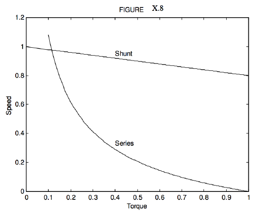
\(\text{FIGURE X.8}\)

The characteristics of the two may be combined in a compound-wound motor, depending on the intended application. For example, a tape-recorder requires constant speed, whereas a car starter requires a high starting torque.