23.6: Forced Damped Oscillator

Let’s drive our damped spring-object system by a sinusoidal force. Suppose that the x - component of the driving force is given by

$$F_{x}(t)=F_{0} \cos (\omega t) \nonumber$$

where $F_{0}$ is called the amplitude (maximum value) and $\omega$ is the driving angular frequency. The force varies between $F_{0}$ and $-F_{0}$ because the cosine function varies between +1 and −1. Define x(t) to be the position of the object with respect to the equilibrium position. The x -component of the force acting on the object is now the sum

$$F_{x}=F_{0} \cos (\omega t)-k x-b \frac{d x}{d t} \nonumber$$

Newton’s Second law in the x -direction becomes

$$F_{0} \cos (\omega t)-k x-b \frac{d x}{d t}=m \frac{d^{2} x}{d t^{2}} \nonumber$$

We can rewrite Equation (23.6.3) as

$$F_{0} \cos (\omega t)=m \frac{d^{2} x}{d t^{2}}+b \frac{d x}{d t}+k x \nonumber$$

We derive the solution to Equation (23.6.4) in Appendix 23E: Solution to the forced Damped Oscillator Equation. The solution to is given by the function

$$x(t)=x_{0} \cos (\omega t+\phi) \nonumber$$

where the amplitude $x_{0}$ is a function of the driving angular frequency ω and is given by

$$x_{0}(\omega)=\frac{F_{0} / m}{\left((b / m)^{2} \omega^{2}+\left(\omega_{0}^{2}-\omega^{2}\right)^{2}\right)^{1 / 2}} \nonumber$$

The phase constant φ is also a function of the driving angular frequency ω and is given by

$$\phi(\omega)=\tan ^{-1}\left(\frac{(b / m) \omega}{\omega^{2}-\omega_{0}^{2}}\right) \nonumber$$

In Equations (23.6.6) and (23.6.7)

$$\omega_{0}=\sqrt{\frac{k}{m}} \nonumber$$

is the natural angular frequency associated with the undriven undamped oscillator. The x -component of the velocity can be found by differentiating Equation (23.6.5),

$$v_{x}(t)=\frac{d x}{d t}(t)=-\omega x_{0} \sin (\omega t+\phi) \nonumber$$

where the amplitude $x_{0}(\omega)$ is given by Equation (23.6.6) and the phase constant $\phi(\omega)$ is given by Equation (23.6.7).

Resonance

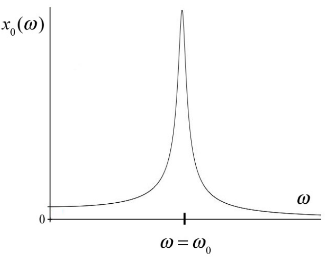
When $b / m<<2 \omega_{0}$ we say that the oscillator is lightly damped. For a lightly-damped driven oscillator, after a transitory period, the position of the object will oscillate with the same angular frequency as the driving force. The plot of amplitude $x_{0}(\omega)$ vs. driving angular frequency ω for a lightly damped forced oscillator is shown in Figure 23.16. If the angular frequency is increased from zero, the amplitude of the $x_{0}(\omega)$ will increase until it reaches a maximum when the angular frequency of the driving force is the same as the natural angular frequency, $\omega_{0}$ associated with the undamped oscillator. This is called resonance. When the driving angular frequency is increased above the natural angular frequency the amplitude of the position oscillations diminishes.

Figure 23.16 Plot of amplitude $x_{0}(\omega)$ vs. driving angular frequency ω for a lightly damped oscillator with $b / m<<2 \omega_{0}$

We can find the angular frequency such that the amplitude $x_{0}(\omega)$ is at a maximum by setting the derivative of Equation (23.6.6) equal to zero,

$$0=\frac{d}{d t} x_{0}(\omega)=-\frac{F_{0}(2 \omega)}{2 m} \frac{\left((b / m)^{2}-2\left(\omega_{0}^{2}-\omega^{2}\right)\right)}{\left((b / m)^{2} \omega^{2}+\left(\omega_{0}^{2}-\omega^{2}\right)^{2}\right)^{3 / 2}} \nonumber$$

This vanishes when

$$\omega=\left(\omega_{0}^{2}-(b / m)^{2} / 2\right)^{1 / 2} \nonumber$$

For the lightly-damped oscillator, $\omega_{0}>>(1 / 2) b / m$, and so the maximum value of the amplitude occurs when

$$\omega \simeq \omega_{0}=(k / m)^{1 / 2} \nonumber$$

The amplitude at resonance is then

$$x_{0}\left(\omega=\omega_{0}\right)=\frac{F_{0}}{b \omega_{0}} \quad \text { (lightly damped) } \nonumber$$

The plot of phase constant $\phi(\omega)$ vs. driving angular frequency ω for a lightly damped forced oscillator is shown in Figure 23.17.

Figure 23.17 Plot of phase constant $\phi(\omega)$ vs. driving angular frequency ω for a lightly damped oscillator with $b / m<<2 \omega_{0}$

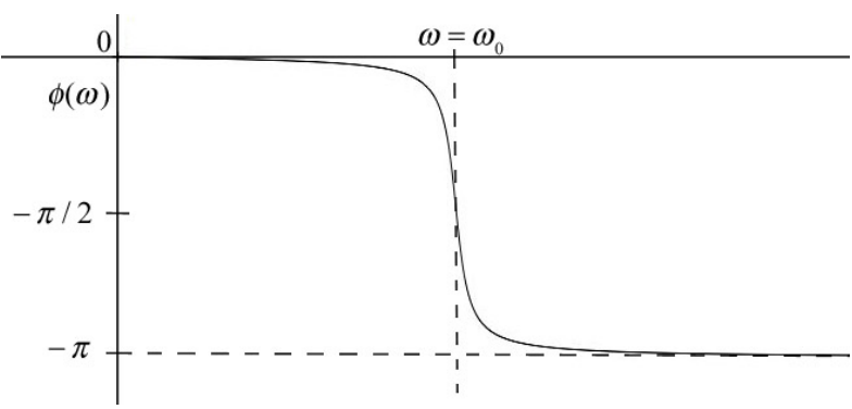
The phase constant at resonance is zero,

$$\phi\left(\omega=\omega_{0}\right)=0 \nonumber$$

At resonance, the x -component of the velocity is given by

$$v_{x}(t)=\frac{d x}{d t}(t)=-\frac{F_{0}}{b} \sin \left(\omega_{0} t\right) \quad \text { (lightly damped) } \nonumber$$

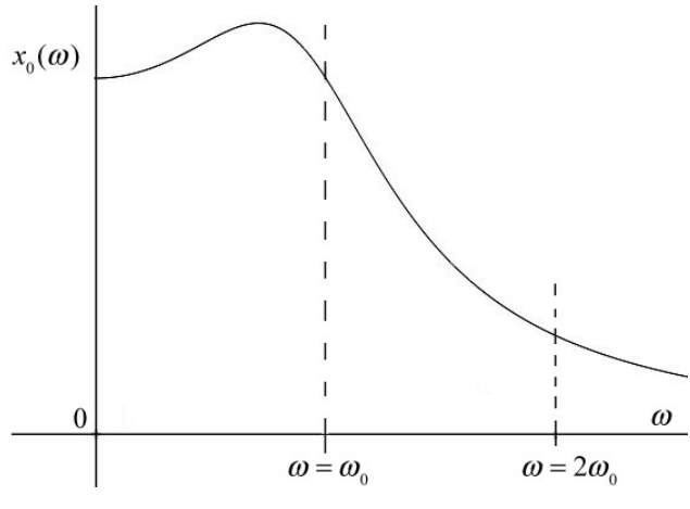
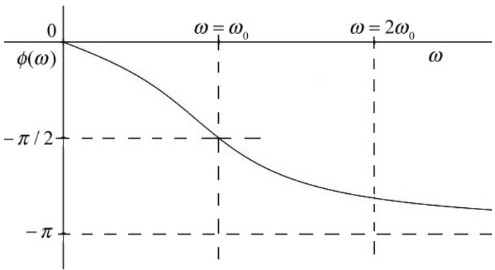
When the oscillator is not lightly damped $\left(b / m \simeq \omega_{0}\right)$, the resonance peak is shifted to the left of $\omega=\omega_{0}$ as shown in the plot of amplitude vs. angular frequency in Figure 23.18. The corresponding plot of phase constant vs. angular frequency for the non-lightly damped oscillator is shown in Figure 23.19.

Figure 23.18 Plot of amplitude vs. angular frequency for lightly-damped driven oscillator where $b / m \simeq \omega_{0}$

Figure 23.19 Plot of phase constant vs. angular frequency for lightly-damped driven oscillator where $b / m \simeq \omega_{0}$

Mechanical Energy

The kinetic energy for the driven damped oscillator is given by

$$K(t)=\frac{1}{2} m v^{2}(t)=\frac{1}{2} m \omega^{2} x_{0}^{2} \sin ^{2}(\omega t+\phi) \nonumber$$

The potential energy is given by

$$U(t)=\frac{1}{2} k x^{2}(t)=\frac{1}{2} k x_{0}^{2} \cos ^{2}(\omega t+\phi) \nonumber$$

The mechanical energy is then

$$E(t)=\frac{1}{2} m v^{2}(t)+\frac{1}{2} k x^{2}(t)=\frac{1}{2} m \omega^{2} x_{0}^{2} \sin ^{2}(\omega t+\phi)+\frac{1}{2} k x_{0}^{2} \cos ^{2}(\omega t+\phi) \nonumber$$

Example 23.5: Time-Averaged Mechanical Energy

The period of one cycle is given by $T=2 \pi / \omega$. Show that

(i) $\frac{1}{T} \int_{0}^{T} \sin ^{2}(\omega t+\phi) d t=\frac{1}{2}$

(ii) $\frac{1}{T} \int_{0}^{T} \cos ^{2}(\omega t+\phi) d t=\frac{1}{2}$

(iii) $\frac{1}{T} \int_{0}^{T} \sin (\omega t) \cos (\omega t) d t=0$

Solution: (i) We use the trigonometric identity

$$\left.\sin ^{2}(\omega t+\phi)\right)=\frac{1}{2}(1-\cos (2(\omega t+\phi)) \nonumber$$

to rewrite the integral in Equation (23.6.19) as

$$\left.\frac{1}{T} \int_{0}^{T} \sin ^{2}(\omega t+\phi)\right) d t=\frac{1}{2 T} \int_{0}^{T}(1-\cos (2(\omega t+\phi)) d t \nonumber$$

Integration yields

$$\begin{array}{l} \frac{1}{2 T} \int_{0}^{T}\left(1-\cos (2(\omega t+\phi)) d t=\frac{1}{2}-\left.\left(\frac{\sin (2(\omega t+\phi))}{2 \omega}\right)\right|_{T=0} ^{T=2 \pi / \omega}\right. \\ =\frac{1}{2}-\left(\frac{\sin (4 \pi+2 \phi)}{2 \omega}-\frac{\sin (2 \phi)}{2 \omega}\right)=\frac{1}{2} \end{array} \nonumber$$

where we used the trigonometric identity that

$$\sin (4 \pi+2 \phi)=\sin (4 \pi) \cos (2 \phi)+\sin (2 \phi) \cos (4 \pi)=\sin (2 \phi) \nonumber$$

proving Equation (23.6.19).

(ii) We use a similar argument starting with the trigonometric identity that

$$\left.\cos ^{2}(\omega t+\phi)\right)=\frac{1}{2}(1+\cos (2(\omega t+\phi)) \nonumber$$

Then

$$\left.\frac{1}{T} \int_{0}^{T} \cos ^{2}(\omega t+\phi)\right) d t=\frac{1}{2 T} \int_{0}^{T}(1+\cos (2(\omega t+\phi)) d t \nonumber$$

Integration yields

$$\begin{array}{l} \frac{1}{2 T} \int_{0}^{T}\left(1+\cos (2(\omega t+\phi)) d t=\frac{1}{2}+\left.\left(\frac{\sin (2(\omega t+\phi))}{2 \omega}\right)\right|_{T=0} ^{T=2 \pi / \omega}\right. \\ =\frac{1}{2}+\left(\frac{\sin (4 \pi+2 \phi)}{2 \omega}-\frac{\sin (2 \phi)}{2 \omega}\right)=\frac{1}{2} \end{array} \nonumber$$

(iii) We first use the trigonometric identity that

$$\sin (\omega t) \cos (\omega t)=\frac{1}{2} \sin (\omega t) \nonumber$$

Then

$$\begin{array}{l} \frac{1}{T} \int_{0}^{T} \sin (\omega t) \cos (\omega t) d t=\frac{1}{T} \int_{0}^{T} \sin (\omega t) d t \\ =-\left.\frac{1}{T} \frac{\cos (\omega t)}{2 \omega}\right|_{0} ^{T}=-\frac{1}{2 \omega T}(1-1)=0 \end{array} \nonumber$$

The values of the integrals in Example 23.5 are called the time-averaged values. We denote the time-average value of a function f(t) over one period by

$$\langle f\rangle \equiv \frac{1}{T} \int_{0}^{T} f(t) d t \nonumber$$

In particular, the time-average kinetic energy as a function of the angular frequency is given by

$$\langle K(\omega)\rangle=\frac{1}{4} m \omega^{2} x_{0}^{2} \nonumber$$

The time-averaged potential energy as a function of the angular frequency is given by

$$\langle U(\omega)\rangle=\frac{1}{4} k x_{0}^{2} \nonumber$$

The time-averaged value of the mechanical energy as a function of the angular frequency is given by

$$\langle E(\omega)\rangle=\frac{1}{4} m \omega^{2} x_{0}^{2}+\frac{1}{4} k x_{0}^{2}=\frac{1}{4}\left(m \omega^{2}+k\right) x_{0}^{2} \nonumber$$

We now substitute Equation (23.6.6) for the amplitude into Equation (23.6.34) yielding

$$\langle E(\omega)\rangle=\frac{F_{0}^{2}}{4 m} \frac{\left(\omega_{0}^{2}+\omega^{2}\right)}{\left((b / m)^{2} \omega^{2}+\left(\omega_{0}^{2}-\omega^{2}\right)^{2}\right)} \nonumber$$

A plot of the time-averaged energy versus angular frequency for the lightly-damped case $\left(b / m<<2 \omega_{0}\right)$ is shown in Figure 23.20.

Figure 23.20). We first substitute $\omega=\omega_{0}$ everywhere in Equation (23.6.35) except the term $\omega_{0}^{2}-\omega^{2}$ that appears in the denominator, yielding

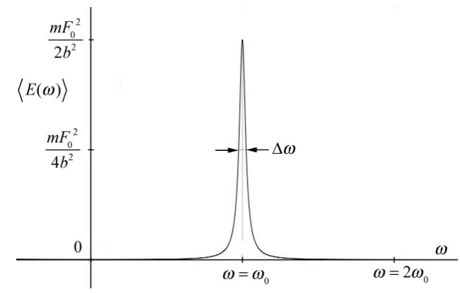
$$\langle E(\omega)\rangle=\frac{F_{0}^{2}}{2 m} \frac{\left(\omega_{0}^{2}\right)}{\left((b / m)^{2} \omega_{0}^{2}+\left(\omega_{0}^{2}-\omega^{2}\right)^{2}\right)} \nonumber$$

We can approximate the term

$$\omega_{0}^{2}-\omega^{2}=\left(\omega_{0}-\omega\right)\left(\omega_{0}+\omega\right) \simeq 2 \omega_{0}\left(\omega_{0}-\omega\right) \nonumber$$

Then Equation (23.6.36) becomes

$$\langle E(\omega)\rangle=\frac{F_{0}^{2}}{2 m} \frac{1}{\left((b / m)^{2}+4\left(\omega_{0}-\omega\right)^{2}\right)} \quad \text { (lightly damped) } \nonumber$$

The right-hand expression of Equation (23.6.38) takes on its maximum value when the denominator has its minimum value. By inspection, this occurs when $\omega=\omega_{0}$. Alternatively, to find the maximum value, we set the derivative of Equation (23.6.35) equal to zero and solve for ω,

$$\begin{array}{l} 0=\frac{d}{d \omega}\langle E(\omega)\rangle=\frac{d}{d \omega} \frac{F_{0}^{2}}{2 m} \frac{1}{\left((b / m)^{2}+4\left(\omega_{0}-\omega\right)^{2}\right)} \\ =\frac{4 F_{0}^{2}}{m} \frac{\left(\omega_{0}-\omega\right)}{\left((b / m)^{2}+4\left(\omega_{0}-\omega\right)^{2}\right)^{2}} \end{array} \nonumber$$

The maximum occurs when occurs at $\omega=\omega_{0}$ and has the value

$$\left\langle E\left(\omega_{0}\right)\right\rangle=\frac{m F_{0}^{2}}{2 b^{2}} \quad(\text { underdamped }) \nonumber$$

The Time-averaged Power

The time-averaged power delivered by the driving force is given by the expression

$$\langle P(\omega)\rangle=\frac{1}{T} \int_{0}^{T} F_{x} v_{x} d t=-\frac{1}{T} \int_{0}^{T} \frac{F_{0}^{2} \omega \cos (\omega t) \sin (\omega t+\phi)}{m\left((b / m)^{2} \omega^{2}+\left(\omega_{0}^{2}-\omega^{2}\right)^{2}\right)^{1 / 2}} d t \nonumber$$

where we used Equation (23.6.1) for the driving force, and Equation (23.6.9) for the x -component of the velocity of the object. We use the trigonometric identity

$$\sin (\omega t+\phi)=\sin (\omega t) \cos (\phi)+\cos (\omega t) \sin (\phi) \nonumber$$

to rewrite the integral in Equation (23.6.41) as two integrals

$$\begin{array}{l} \langle P(\omega)\rangle=-\frac{1}{T} \int_{0}^{T} \frac{F_{0}^{2} \omega \cos (\omega t) \sin (\omega t) \cos (\phi)}{m\left((b / m)^{2} \omega^{2}+\left(\omega_{0}^{2}-\omega^{2}\right)^{2}\right)^{1 / 2}} d t \\ -\frac{1}{T} \int_{0}^{T} \frac{F_{0}^{2} \omega \cos ^{2}(\omega t) \sin (\phi)}{m\left((b / m)^{2} \omega^{2}+\left(\omega_{0}^{2}-\omega^{2}\right)^{2}\right)^{1 / 2}} d t \end{array} \nonumber$$

Using the time-averaged results from Example 23.5, we see that the first term in Equation (23.6.43) is zero and the second term becomes

$$\langle P(\omega)\rangle=\frac{F_{0}^{2} \omega \sin (\phi)}{2 m\left((b / m)^{2} \omega^{2}+\left(\omega_{0}^{2}-\omega^{2}\right)^{2}\right)^{1 / 2}} \nonumber$$

For the underdamped driven oscillator, we make the same approximations in Equation (23.6.44) that we made for the time-averaged energy. In the term in the numerator and the

term on the left in the denominator, we set $\omega=\omega_{0}$, and we use Equation (23.6.37) in the term on the right in the denominator yielding

\[ \langle P(\omega)\rangle=\frac{F_{0}^{2} \sin (\phi)}{2 m\left((b / m)^{2}+2\left(\omega_{0}-\omega\right)\right)^{1 / 2}}(underdamped)\end{equation}

The time-averaged power dissipated by the resistive force is given by

$$\begin{array}{l} \left\langle P_{\mathrm{dis}}(\omega)\right\rangle=\frac{1}{T} \int_{0}^{T}\left(F_{x}\right)_{\mathrm{dis}} v_{x} d t=-\frac{1}{T} \int_{0}^{T} b v_{x}^{2} d t=\frac{1}{T} \int_{0}^{T} \frac{F_{0}^{2} \omega^{2} \sin ^{2}(\omega t+\phi) d t}{m^{2}\left((b / m)^{2} \omega^{2}+\left(\omega_{0}^{2}-\omega^{2}\right)^{2}\right)} \\ =\frac{F_{0}^{2} \omega^{2} d t}{2 m^{2}\left((b / m)^{2} \omega^{2}+\left(\omega_{0}^{2}-\omega^{2}\right)^{2}\right)} \end{array} \nonumber$$

where we used Equation (23.5.1) for the dissipative force, Equation (23.6.9) for the x -component of the velocity of the object, and Equation (23.6.19) for the time-averaging.

Quality Factor

The plot of the time-averaged energy vs. the driving angular frequency for the underdamped oscullator has a width, $\Delta \omega$ (Figure 23.20). One way to characterize this width is to define $\Delta \omega=\omega_{+}-\omega_{-}$, where $\omega_{\pm}$ are the values of the angular frequency such that time-averaged energy is equal to one half its maximum value

$$\left\langle E\left(\omega_{\pm}\right)\right\rangle=\frac{1}{2}\left\langle E\left(\omega_{0}\right)\right\rangle=\frac{m F_{0}^{2}}{4 b^{2}} \nonumber$$

The quantity $\Delta \omega$ is called the line width at half energy maximum also known as the resonance width. We can now solve for $\omega_{\pm}$ by setting

$$\left\langle E\left(\omega_{\pm}\right)\right\rangle=\frac{F_{0}^{2}}{2 m} \frac{1}{\left((b / m)^{2}+4\left(\omega_{0}-\omega_{\pm}\right)^{2}\right)}=\frac{m F_{0}^{2}}{4 b^{2}} \nonumber$$

yielding the condition that

$$(b / m)^{2}=4\left(\omega_{0}-\omega_{\pm}\right)^{2} \nonumber$$

Taking square roots of Equation (23.6.49) yields

$$\mp(b / 2 m)=\omega_{0}-\omega_{\pm} \nonumber$$

Therefore

$$\omega_{\pm}=\omega_{0} \pm(b / 2 m) \nonumber$$

The half-width is then

$$\Delta \omega=\omega_{+}-\omega_{-}=\left(\omega_{0}+(b / 2 m)\right)-\left(\omega_{0}-(b / 2 m)\right)=b / m \nonumber$$

We define the quality Q of the resonance as the ratio of the resonant angular frequency to the line width,

$$Q=\frac{\omega_{0}}{\Delta \omega}=\frac{\omega_{0}}{b / m} \nonumber$$

Figure 23.21 Plot of time-averaged energy vs. angular frequency for different values of $b / m$

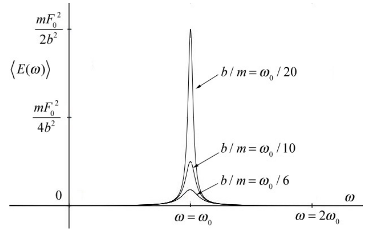
In Figure 23.21 we plot the time-averaged energy vs. angular frequency for several different values of the quality factor Q = 10, 5, and 3. Recall that this was the same result that we had for the quality of the free oscillations of the damped oscillator, Equation (23.5.16) (because we chose the factor $\pi$ in Equation (23.5.16)).