5.1: Free and Forced Oscillations

In Sec. $3.2$ we briefly discussed oscillations in a keystone Hamiltonian system - a 1D harmonic oscillator described by a very simple Lagrangian ${ }^{1}$

$$L \equiv T(\dot{q})-U(q)=\frac{m}{2} \dot{q}^{2}-\frac{\kappa}{2} q^{2},$$ whose Lagrange equation of motion, ${ }^{2}$

$\begin{aligned}&\text { Harmonic } \\&\text { oscillator: } \\&\text { equation }\end{aligned} \quad m \ddot{q}+\kappa q=0, \quad$ i.e. $\ddot{q}+\omega_{0}^{2} q=0, \quad$ with $\omega_{0}^{2} \equiv \frac{\kappa}{m} \geq 0$,

is a linear homogeneous differential equation. Its general solution is given by (3.16), which is frequently recast into another, amplitude-phase form:

$$q(t)=u \cos \omega_{0} t+v \sin \omega_{0} t=A \cos \left(\omega_{0} t-\varphi\right),$$ where $A$ is the amplitude and $\varphi$ the phase of the oscillations, which are determined by the initial conditions. Mathematically, it is frequently easier to work with sinusoidal functions as complex exponents, by rewriting the last form of Eq. (3a) in one more form: $^{3}$ $$q(t)=\operatorname{Re}\left[A e^{-i\left(\omega_{0} t-\varphi\right)}\right]=\operatorname{Re}\left[a e^{-i \omega_{0} t}\right],$$ $$a \equiv A e^{i \varphi}, \quad|a|=A, \quad \operatorname{Re} a=A \cos \varphi=u, \quad \operatorname{Im} a=A \sin \varphi=v .$$ For an autonomous, Hamiltonian oscillator, Eq. (3) gives the full classical description of its dynamics. However, it is important to understand that this free-oscillation solution, with a constant amplitude $A$, is due to the conservation of the energy $E \equiv T+U=\kappa A^{2} / 2$ of the oscillator. If its energy changes for any reason, the description needs to be generalized.

First of all, if the energy leaks out of the oscillator to its environment (the effect usually called the energy dissipation), the free oscillations decay with time. The simplest model of this effect is represented by an additional linear drag (or "kinematic friction") force, proportional to the generalized velocity and directed opposite to it:

$$F_{v}=-\eta \dot{q},$$ where constant $\eta$ is called the drag coefficient. ${ }^{4}$ The inclusion of this force modifies the equation of motion (2) to become $$m \ddot{q}+\eta \dot{q}+\kappa q=0 .$$ This equation is frequently rewritten in the form $$\ddot{q}+2 \delta \ddot{q}+\omega_{0}^{2} q=0, \quad \text { with } \delta \equiv \frac{\eta}{2 m},$$ where the parameter $\delta$ is called the damping coefficient (or just "damping"). Note that Eq. (6) is still a linear homogeneous second-order differential equation, and its general solution still has the form of the sum (3.13) of two exponents of the type $\exp \{\lambda t\}$, with arbitrary pre-exponential coefficients. Plugging such an exponent into Eq. (6), we get the following algebraic characteristic equation for $\lambda$ : $$\lambda^{2}+2 \delta \lambda+\omega_{0}^{2}=0 .$$ Solving this quadratic equation, we get $$\lambda_{\pm}=-\delta \pm i \omega_{0}^{\prime}, \quad \text { where } \omega_{0}^{\prime} \equiv\left(\omega_{0}^{2}-\delta^{2}\right)^{1 / 2},$$ so that for not very high damping $\left(\delta<\omega_{0}\right)^{5}$ we get the following generalization of Eq. (3): $$q_{\text {free }}(t)=c_{+} e^{\lambda_{+} t}+c_{-} e^{\lambda_{-} t}=\left(u_{0} \cos \omega_{0}^{\prime} t+v_{0} \sin \omega_{0}^{\prime} t\right) e^{-\delta t}=A_{0} e^{-\delta t} \cos \left(\omega_{0}^{\prime} t-\varphi_{0}\right) .$$ The result shows that, besides a certain correction to the free oscillation frequency (which is very small in the most interesting low damping limit, $\delta<<\omega_{0}$ ), the energy dissipation leads to an exponential decay of oscillation amplitude with the time constant $\tau=1 / \delta$: $$A=A_{0} e^{-t / \tau}, \quad \text { where } \tau \equiv \frac{1}{\delta}=\frac{2 m}{\eta}$$ A very popular dimensionless measure of damping is the so-called quality factor $Q$ (or just the $Q$-factor ) that is defined as $\omega_{0} / 2 \delta$, and may be rewritten in several other useful forms: $$Q \equiv \frac{\omega_{0}}{2 \delta}=\frac{m \omega_{0}}{\eta}=\frac{(m \kappa)^{1 / 2}}{\eta}=\pi \frac{\tau}{\tau}=\frac{\omega_{0} \tau}{2},$$ where $\tau=2 \pi / \omega_{0}$ is the oscillation period in the absence of damping - see Eq. (3.29). Since the oscillation energy $E$ is proportional to $A^{2}$, i.e. decays as $\exp \{-2 t / \tau\}$, with the time constant $\tau / 2$, the last form of Eq. (11) may be used to rewrite the $Q$-factor in one more form: $$Q=\omega_{0} \frac{E}{(-\dot{E})} \equiv \omega_{0} \frac{E}{\mathscr{P}},$$ where $\mathscr{P}$ is the dissipation power. (Two other practical ways to measure $Q$ will be discussed below.) The range of $Q$-factors of important oscillators is very broad, all the way from $Q \sim 10$ for a human leg (with relaxed muscles), to $Q \sim 10^{4}$ of the quartz crystals used in electronic clocks and watches, all the way up to $Q \sim 10^{12}$ for carefully designed microwave cavities with superconducting walls.

In contrast to the decaying free oscillations, the forced oscillations, induced by an external force $F(t)$, may maintain their amplitude (and hence energy) infinitely, even at non-zero damping. This process may be described using a still linear but now inhomogeneous differential equation

$$m \ddot{q}+\eta \dot{q}+\kappa q=F(t),$$ or, more conveniently for analysis, the following generalization of Eq. (6b):

$\begin{aligned}&\text { Forced } \\&\text { oscillator } \\&\text { with } \\&\text { damping }\end{aligned} \quad \ddot{q}+2 \delta \dot{q}+\omega_{0}^{2} q=f(t), \quad$ where $f(t) \equiv F(t) / m .$

For a mechanical linear, dissipative $1 \mathrm{D}$ oscillator $(6)$, under the effect of an additional external force $F(t)$, Eq. (13a) is just an expression of the $2^{\text {nd }}$ Newton law. However, according to Eq. (1.41), Eq. (13) is valid for any dissipative, linear 6 1D system whose Gibbs potential energy $(1.39)$ has the form $U_{\mathrm{G}}(q, t)=$ $\kappa q^{2} / 2-F(t) q$.

The forced-oscillation solutions may be analyzed by two mathematically equivalent methods whose relative convenience depends on the character of function $f(t)$.

(i) Frequency domain. Representing the function $f(t)$ as a Fourier sum of sinusoidal harmonics: $^{7}$

$$f(t)=\sum_{\omega} f_{\omega} e^{-i \omega t},$$ and using the linearity of Eq. (13), we may represent its general solution as a sum of the decaying free oscillations (9) with the frequency $\omega_{0}^{\prime}$, independent of the function $f(t)$, and forced oscillations due to each of the Fourier components of the force: $^{8}$ $$q(t)=q_{\text {free }}(t)+q_{\text {forced }}(t), \quad q_{\text {forced }}(t)=\sum_{\omega} a_{\omega} e^{-i \omega t}$$ Plugging Eq. (15) into Eq. (13), and requiring the factors before each $e^{-i \omega t}$ on both sides to be equal, we get $$a_{\omega}=f_{\omega} \chi(\omega),$$ where the complex function $\chi(\omega)$, in our particular case equal to $$\chi(\omega)=\frac{1}{\left(\omega_{0}^{2}-\omega^{2}\right)-2 i \omega \delta},$$ is called either the response function or (especially for non-mechanical oscillators) the generalized susceptibility. From here, and Eq. (4), the amplitude of the oscillations under the effect of a sinusoidal force is $$A_{\omega} \equiv\left|a_{\omega}\right|=\left|f_{\omega} \| \chi(\omega)\right|, \quad \text { with }|\chi(\omega)|=\frac{1}{\left[\left(\omega_{0}^{2}-\omega^{2}\right)^{2}+(2 \omega \delta)^{2}\right]^{1 / 2}}$$ This formula describes, in particular, an increase of the oscillation amplitude $A_{\omega}$ at $\omega \rightarrow \omega_{0}-$ see the left panel in Figure 1. In particular, at the exact equality of these two frequencies, $$|\chi(\omega)|_{\omega=\omega_{0}}=\frac{1}{2 \omega_{0} \delta},$$ so that, according to Eq. (11), the ratio of the response magnitudes at $\omega=\omega_{0}$ and $\omega=0\left(|\chi(\omega)|_{\omega=0}=\right.$ $1 / \omega_{0}{ }^{2}$ ) is exactly equal to the $Q$-factor of the oscillator. Thus, the response increase is especially strong in the low damping limit $\left(\delta<<\omega_{0}\right.$, i.e. $\left.Q>>1\right)$; moreover at $Q \rightarrow \infty$ and $\omega \rightarrow \omega_{0}$ the response diverges. (This fact is very useful for the methods to be discussed later in this section.) This is the classical description of the famous phenomenon of resonance, so ubiquitous in physics.

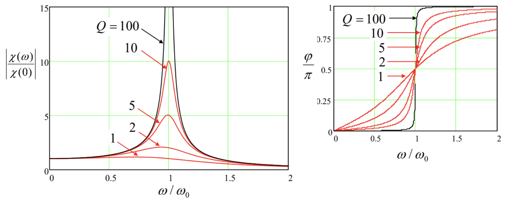
Figure 5.1. Resonance in the linear oscillator, for several values of $Q$.

Due to the increase of the resonance peak height, its width is inversely proportional to $Q$. Quantitatively, in the most interesting low-damping limit, i.e. at $Q>>1$, the reciprocal $Q$-factor gives the normalized value of the so-called full-width at half-maximum (FWHM) of the resonance curve: $^{9}$

$$\frac{\Delta \omega}{\omega_{0}}=\frac{1}{Q} .$$ Indeed, this $\Delta \omega$ is defined as the difference $\left(\omega_{+}-\omega_{-}\right)$between the two values of $\omega$ at that the square of the oscillator response function, $|\chi(\omega)|^{2}$ (which is proportional to the oscillation energy), equals a half of its resonance value (19). In the low damping limit, both these points are very close to $\omega_{0}$, so that in the linear approximation in $\left|\omega^{-} \omega_{0}\right|<<\omega_{0}$, we may write $\left(\omega_{0}{ }^{2-} \omega^{2}\right) \equiv-\left(\omega+\omega_{0}\right)\left(\omega^{-} \omega_{0}\right) \approx-2 \omega \xi \approx-2 \omega_{0} \xi$, where $$\xi \equiv \omega-\omega_{0}$$ is a very convenient parameter called detuning, which will be repeatedly used later in this chapter. In this approximation, the second of Eqs. (18) is reduced to ${ }^{10}$ $$|\chi(\omega)|^{2}=\frac{1}{4 \omega_{0}^{2}\left(\delta^{2}+\xi^{2}\right)} .$$ As a result, the points $\omega_{\pm}$correspond to $\xi^{2}=\delta^{2}$, i.e. $\omega_{\pm}=\omega_{0} \pm \delta=\omega_{0}(1 \pm 1 / 2 Q)$, so that $\Delta \omega \equiv \omega_{+}-\omega_{-}=$ $\omega_{0} / Q$, thus proving Eq. (20).

(ii) Time domain. Returning to arbitrary external force $f(t)$, one may argue that Eqs. (9), (15)-(17) provide a full solution of the forced oscillation problem even in this general case. This is formally correct, but this solution may be very inconvenient if the external force is far from a sinusoidal function of time, especially if it is not periodic at all. In this case, we should first calculate the complex amplitudes $f_{\omega}$ participating in the Fourier sum (14). In the general case of a non-periodic $f(t)$, this is actually the Fourier integral, ${ }^{11}$

$$f(t)=\int_{-\infty}^{+\infty} f_{\omega} e^{-i \omega t} d t,$$ so that $f_{\omega}$ should be calculated using the reciprocal Fourier transform, $$f_{\omega}=\frac{1}{2 \pi} \int_{-\infty}^{+\infty} f\left(t^{\prime}\right) e^{i \omega t^{\prime}} d t^{\prime}$$ Now we may use Eq. (16) for each Fourier component of the resulting forced oscillations, and rewrite the last of Eqs. (15) as $$\begin{aligned} q_{\text {forced }}(t) &=\int_{-\infty}^{+\infty} a_{\omega} e^{-i \omega t} d \omega=\int_{-\infty}^{+\infty} \chi(\omega) f_{\omega} e^{-i \omega t} d \omega=\int_{-\infty}^{+\infty} d \omega \chi(\omega) \frac{1}{2 \pi} \int_{-\infty}^{+\infty} d t^{\prime} f\left(t^{\prime}\right) e^{i \omega\left(t^{\prime}-t\right)} \\ &=\int_{-\infty}^{+\infty} d t^{\prime} f\left(t^{\prime}\right)\left[\frac{1}{2 \pi} \int_{-\infty}^{+\infty} d \omega \chi(\omega) e^{i \omega\left(t^{\prime}-t\right)}\right] \end{aligned}$$ with the response function $\chi(\omega)$ given, in our case, by Eq. (17). Besides requiring two integrations, Eq. (25) is conceptually uncomforting: it seems to indicate that the oscillator’s coordinate at time $t$ depends not only on the external force exerted at earlier times $t$ ’ $<t$, but also at future times. This would contradict one of the most fundamental principles of physics (and indeed, science as a whole), the causality: no effect may precede its cause.

Fortunately, a straightforward calculation (left for the reader’s exercise) shows that the response function (17) satisfies the following rule: ${ }^{12}$

$$\int_{-\infty}^{+\infty} \chi(\omega) e^{-i \omega \tau} d \omega=0, \quad \text { for } \tau<0 .$$ This fact allows the last form of Eq. (25) to be rewritten in either of the following equivalent forms: $$q_{\text {forced }}(t)=\int_{-\infty}^{t} f\left(t^{\prime}\right) G\left(t-t^{\prime}\right) d t^{\prime} \equiv \int_{0}^{\infty} f(t-\tau) G(\tau) d \tau,$$ where $G(\tau)$, defined as the Fourier transform of the response function, $$G(\tau) \equiv \frac{1}{2 \pi} \int_{-\infty}^{+\infty} \chi(\omega) e^{-i \omega \tau} d \omega,$$ is called the (temporal) Green’s function of the system. According to Eq. (26), $G(\tau)=0$ for all $\tau<0$.

While the second form of Eq. (27) is frequently more convenient for calculations, its first form is more suitable for physical interpretation of the Green’s function. Indeed, let us consider the particular case when the force is a delta function

$$f(t)=\delta\left(t-t^{\prime}\right), \quad \text { with } t^{\prime}<t \text {, i.e. } \tau \equiv t-t^{\prime}>0 \text {, }$$ representing an ultimately short pulse at the moment $t$ ’, with unit "area" $\int f(t) d t$. Substituting Eq. (29a) into Eq. (27), ${ }^{13}$ we get $$q(t)=G\left(t-t^{\prime}\right) .$$ Thus the Green’s function $G\left(t-t^{\prime}\right)$ is just the oscillator’s response, as measured at time $t$, to a short force pulse of unit "area", exerted at time $t$ ’. Hence Eq. (27) expresses the linear superposition principle in the time domain: the full effect of the force $f(t)$ on a linear system is a sum of effects of short pulses of duration $d t$ ’ and magnitude $f\left(t^{\prime}\right)$, each with its own "weight" $G\left(t-t^{\prime}\right)$ - see Figure 2 .

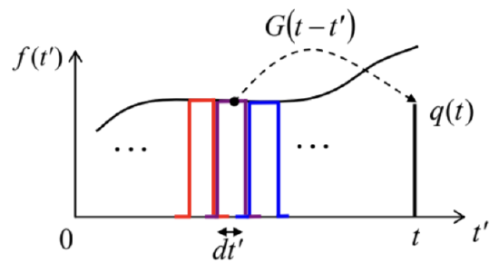
Figure 5.2. A schematic, finite-interval representation of a force $f(t)$ as a sum of short pulses at all times $t^{\prime}<t$, and their contributions to the linear system’s response $q(t)$, as given by Eq. (27).

This picture may be used for the calculation of Green’s function for our particular system. Indeed, Eqs. (29)-(30) mean that $G(\tau)$ is just the solution of the differential equation of motion of the system, in our case, Eq. (13), with the replacement $t \rightarrow \tau$, and a $\delta$-functional right-hand side:

$$\frac{d^{2} G(\tau)}{d \tau^{2}}+2 \delta \frac{d G(\tau)}{d \tau}+\omega_{0}^{2} G(\tau)=\delta(\tau) .$$ Since Eqs. (27) describes only the second term in Eq. (15), i.e. only the forced, rather than free oscillations, we have to exclude the latter by solving Eq. (31) with zero initial conditions: $$G(-0)=\frac{d G}{d \tau}(-0)=0,$$ where $\tau=-0$ means the instant immediately preceding $\tau=0$.

This calculation may be simplified even further. Let us integrate both sides of Eq. (31) over an infinitesimal interval including the origin, e.g. [- $d \tau / 2,+d \tau / 2]$, and then follow the limit $d \tau \rightarrow 0$. Since the Green’s function has to be continuous because of its physical sense as the (generalized) coordinate, all terms on the left-hand side but the first one vanish, while the first term yields $d G /\left.d \tau\right|_{+0}-d G /\left.d \tau\right|_{-0}$. Due to the second of Eqs. (32), the last of these two derivatives equals zero, while the right-hand side of Eq. (31) yields 1 upon the integration. Thus, the function $G(\tau)$ may be calculated for $\tau>0$ (i.e. for all times when it is different from zero) by solving the homogeneous version of the system’s equation of motion for $\tau>0$, with the following special initial conditions:

$$G(0)=0, \quad \frac{d G}{d \tau}(0)=1 .$$ This approach gives us a convenient way for the calculation of Green’s functions of linear systems. In particular for the oscillator with not very high damping $\left(\delta<\omega_{0}\right.$, i.e. $\left.Q>1 / 2\right)$, imposing the boundary conditions $(33)$ on the homogeneous equation’s solution $(9)$, we immediately get $$G(\tau)=\frac{1}{\omega_{0}{ }^{\prime}} e^{-\delta \tau} \sin \omega_{0}{ }^{\prime} \tau$$ (The same result may be obtained directly from Eq. (28) with the response function $\chi(\omega)$ given by Eq. (19). This way is, however, a little bit more cumbersome, and is left for the reader’s exercise.)

Relations (27) and (34) provide a very convenient recipe for solving many forced oscillations problems. As a very simple example, let us calculate the transient process in an oscillator under the effect of a constant force being turned on at $t=0$, i.e. proportional to the theta-function of time:

$$f(t)=f_{0} \theta(t) \equiv \begin{cases}0, & \text { for } t<0, \\ f_{0}, & \text { for } t>0,\end{cases}$$ provided that at $t<0$ the oscillator was at rest, so that in Eq. (15), $q_{\text {free }}(t) \equiv 0$. Then the second form of Eq. (27), and Eq. (34), yield $$q(t)=\int_{0}^{\infty} f(t-\tau) G(\tau) d \tau=f_{0} \int_{0}^{t} \frac{1}{\omega_{0}{ }^{\prime}} e^{-\delta \tau} \sin \omega_{0}{ }^{\prime} \tau d \tau .$$ The simplest way to work out such integrals is to represent the sine function under it as the imaginary part of $\exp \left\{i \omega_{0}^{\prime} t\right\}$, and merge the two exponents, getting $$q(t)=f_{0} \frac{1}{\omega_{0}^{\prime}} \operatorname{Im}\left[\frac{1}{-\delta+i \omega_{0}^{\prime}} e^{-\delta \tau+i \omega_{0}^{\prime} \tau}\right]_{0}^{t}=\frac{F_{0}}{k}\left[1-e^{-\delta t}\left(\cos \omega_{0}^{\prime} t+\frac{\delta}{\omega_{0}^{\prime}} \sin \omega_{0}^{\prime} t\right)\right]$$

This result, plotted in Figure 3, is rather natural: it describes nothing more than the transient from the initial position $q=0$ to the new equilibrium position $q_{0}=f_{0} / \omega_{0}{ }^{2}=F_{0} / \kappa$, accompanied by decaying oscillations. For this particular simple function $f(t)$, the same result might be also obtained by introducing a new variable $\widetilde{q}(t) \equiv q(t)-q_{0}$ and solving the resulting homogeneous equation for $\widetilde{q}$ (with appropriate initial condition $\ \widetilde{q}(0)=-q_{0}$. However, for more complicated functions $\ f(t)$ the Green’s function approach is irreplaceable.

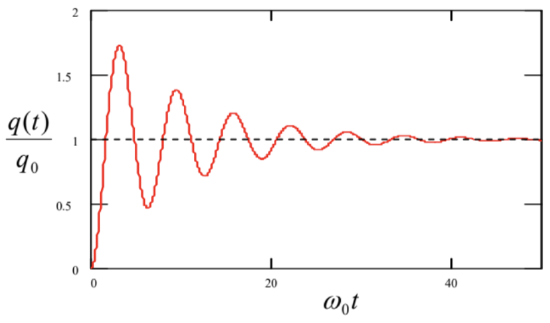
Figure 5.3. The transient process in a linear oscillator, induced by a step-like force $f(t)$, for the particular case $\delta / \omega_{0}=0.1$ (i.e., $Q=5$ ).

Note that for any particular linear system, its Green’s function should be calculated only once, and then may be repeatedly used in Eq. (27) to calculate the system response to various external forces either analytically or numerically. This property makes the Green’s function approach very popular in many other fields of physics $-$ with the corresponding generalization or re-definition of the function. ${ }^{14}$

---

${ }^{1}$ For the notation brevity, in this chapter I will drop indices "ef" in the energy components $T$ and $U$, and parameters like $m, \kappa$, etc. However, the reader should still remember that $T$ and $U$ do not necessarily coincide with the actual kinetic and potential energies (even if those energies may be uniquely identified) - see Sec. 3.1.

${ }^{2} \omega_{0}$ is usually called the own frequency of the oscillator. In quantum mechanics, the Germanized version of the same term, eigenfrequency, is used more. In this series, I will use either of the terms, depending on the context.

${ }^{3}$ Note that this is the so-called physics convention. Most engineering texts use the opposite sign in the imaginary exponent, $\exp \{-i \omega t\} \rightarrow \exp \{i \omega t\}$, with the corresponding sign implications for intermediate formulas, but (of course) similar final results for real variables.

${ }^{4}$ Here Eq. (5) is treated as a phenomenological model, but in statistical mechanics, such dissipative term may be derived as an average force exerted upon a system by its environment, at very general assumptions. As discussed in detail elsewhere in this series (SM Chapter 5 and QM Chapter 7), due to the numerous degrees of freedom of a typical environment (think about the molecules of air surrounding the usual mechanical pendulum), its force also has a random component; as a result, the dissipation is fundamentally related to fluctuations. The latter effects may be neglected (as they are in this course) only if $E$ is much higher than the energy scale of the random fluctuations of the oscillator - in the thermal equilibrium at temperature $T$, the larger of $k_{\mathrm{B}} T$ and $\hbar \omega_{0} / 2$.

${ }^{5}$ Systems with high damping $\left(\delta>\omega_{0}\right)$ can hardly be called oscillators, and though they are used in engineering and physics experiment (e.g., for the shock, vibration, and sound isolation), for their detailed discussion I have to refer the interested reader to special literature - see, e.g., C. Harris and A. Piersol, Shock and Vibration Handbook, $5^{\text {th }}$ ed., McGraw Hill, 2002. Let me only note that dynamics of systems with very high damping $(\delta \gg>$ $\omega_{0}$ ) has two very different time scales: a relatively short "momentum relaxation time" $1 / \lambda \approx 1 / 2 \delta=m / \eta$, and a much longer "coordinate relaxation time" $1 / \lambda_{+} \approx 2 \delta / \omega_{0}{ }^{2}=\eta / \kappa$.

${ }^{6}$ This is a very unfortunate, but common jargon, meaning "the system described by linear equations of motion".

${ }^{7}$ Here, in contrast to Eq. (3b), we may drop the operator Re, assuming that $f_{-\omega}=f_{\omega}{ }^{*}$, so that the imaginary components of the sum compensate each other.

${ }^{8}$ In physics, this mathematical property of linear equations is frequently called the linear superposition principle.

${ }^{9}$ Note that the phase shift $\varphi \equiv \arg [\chi(\omega)]$ between the oscillations and the external force (see the right panel in Figure 1) makes its steepest change, by $\pi / 2$, within the same frequency interval $\Delta \omega$.

${ }^{10}$ Such function of frequency is met in many branches of science, frequently under special names, including the "Cauchy distribution", "the Lorentz function" (or "Lorentzian line", or "Lorentzian distribution"), "the BreitWigner function" (or "the Breit-Wigner distribution"), etc.

${ }^{11}$ Let me hope that the reader knows that Eq. (23) may be used for periodic functions as well; in such a case, $f_{\omega}$ is a set of equidistant delta functions. (A reminder of the basic properties of the Dirac $\delta$-function may be found, for example, in MA Sec. 14.)

${ }^{12}$ Eq. (26) remains true for any linear physical systems in which $f(t)$ represents a cause, and $q(t)$ its effect. Following tradition, I discuss the frequency-domain expression of this causality relation (called the KramersKronig relations) in the Classical Electrodynamics part of this lecture series - see EM Sec. 7.2.

${ }^{13}$ Technically, for this integration, $t$ ’ in Eq. (27) should be temporarily replaced with another letter, say $t$ ".

${ }^{14}$ See, e.g., EM Sec. 2.7, and QM Sec. $2.2 .$