
5.2: Weakly Nonlinear Oscillations


- Last updated
- Jan 27, 2022
- Save as PDF

( \newcommand{\kernel}{\mathrm{null}\,}\)
In comparison with systems discussed in the last section, which are described by linear differential equations with constant coefficients and thus allow a complete and exact analytical solution, oscillations in nonlinear systems (very unfortunately but commonly called nonlinear oscillations) present a complex and, generally, analytically intractable problem. However, much insight on possible processes in such systems may be gained from a discussion of an important case of weakly nonlinear systems, which may be explored analytically. An important example of such systems is given by an anharmonic oscillator - a 1D system whose higher terms in the potential expansion (3.10) cannot be neglected, but are small and may be accounted for approximately. If, in addition, damping is low (or negligible), and the external harmonic force exerted on the system is not too large, the equation of motion is a slightly modified version of Eq. (13): ¨q+ω2q=f(t,q,˙q,…), where ω≈ω0 is the anticipated frequency of oscillations (whose choice is to a certain extent arbitrary see below), and the right-hand side f is small (say, scales as some small dimensionless parameter ε<< 1), and may be considered as a small perturbation.
Since at ε=0 this equation has the sinusoidal solution given by Eq. (3), one might naïvely think that at a nonzero but small ε, the approximate solution to Eq. (38) should be sought in the form q(t)=q(0)+q(1)+q(2)+…, where q(n)∝εn, with q(0)=Acos(ω0t−φ)∝ε0. This is a good example of apparently impeccable mathematical reasoning that would lead to a very inefficient procedure. Indeed, let us apply it to the problem we already know the exact solution for, namely the free oscillations in a linear but damped oscillator, for this occasion assuming the damping to be very low, δ/ω0∼ε<<1. The corresponding equation of motion, Eq. (6), may be represented in form (38) if we take ω=ω0 and f=−2δ˙q, with δ∝ε. The naïve approach described above would allow us to find small corrections, of the order of δ, to the free, non-decaying oscillations Acos(ω0t−φ). However, we already know from Eq. (9) that the main effect of damping is a gradual decrease of the free oscillation amplitude to zero, i.e. a very large change of the amplitude, though at low damping, δ<<ω0, this decay takes large time t∼τ>>1/ω0. Hence, if we want our approximate method to be productive (i.e. to work at all time scales, in particular for forced oscillations with stationary amplitude and phase), we need to account for the fact that the small righthand side of Eq. (38) may eventually lead to essential changes of oscillation’s amplitude A (and sometimes, as we will see below, also of oscillation’s phase φ ) at large times, because of the slowly accumulating effects of the small perturbation. 15
This goal may be achieved 16 by the account of these slow changes already in the " 0th approximation", i.e. the basic part of the solution in the expansion (39): q(0)=A(t)cos[ωt−φ(t)], with ˙A,˙φ→0 at ε→0 (It is evident that Eq. (9) is a particular case of this form.) Let me discuss this approach using a simple but representative example of a dissipative (but high- Q ) pendulum driven by a weak sinusoidal external force with a nearly-resonant frequency: ¨q+2δ¨q+ω20sinq=f0cosωt, with |ω−ω0|,δ<<ω0, and the force amplitude f0 so small that |q|<<1 at all times. From what we know about the forced oscillations from Sec. 1, in this case it is natural to identify ω on the left-hand side of Eq. (38) with the force’s frequency. Expanding sinq into the Taylor series in small q, keeping only the first two terms of this expansion, and moving all small terms to the right-hand side, we can rewrite Eq. (42) in the following popular form (38): 17 ¨q+ω2q=−2δ¨q+2ξωq+αq3+f0cosωt≡f(t,q,˙q). Here α=ω20/6 in the case of the pendulum (though the calculations below will be valid for any α ), and the second term on the right-hand side was obtained using the approximation already employed in Sec. 1:(ω2−ω20)q≈2ω(ω−ω0)q=2ωξq, where ξ≡ω−ω0 is the detuning parameter that was already used earlier - see Eq. (21).
Now, following the general recipe expressed by Eqs. (39) and (41), in the 1st approximation in f ∝ε we may look for the solution to Eq. (43) in the following form: 18 q(t)=AcosΨ+q(1)(t), where Ψ≡ωt−φ,q(1)∼ε. Let us plug this solution into both parts of Eq. (43), keeping only the terms of the first order in ε. Thanks to our (smart :-) choice of ω on the left-hand side of that equation, the two zero-order terms in that part cancel each other. Moreover, since each term on the right-hand side of Eq. (43) is already of the order of ε, we may drop q(1)∝ε from the substitution into that part at all, because this would give us only terms O(ε2) or higher. As a result, we get the following approximate equation: ¨q(1)+ω2q(1)=f(0)≡−2δddt(AcosΨ)+2ξω(AcosΨ)+α(AcosΨ)3+f0cosωt. According to Eq. (41), generally, A and φ should be considered (slow) functions of time. However, let us leave the analyses of the transient process and system’s stability until the next section, and use Eq. (45) to find stationary oscillations in the system, that are established after an initial transient. For that limited task, we may take A= const, φ= const, so that q(0) represents sinusoidal oscillations of frequency ω. Sorting the terms on the right-hand side according to their time dependence, 19 we see that it has terms with frequencies ω and 3ω : f(0)=(2ξωA+34αA3+f0cosφ)cosΨ+(2δωA−f0sinφ)sinΨ+14αA3cos3Ψ. Now comes the main punch of the van der Pol approach: mathematically, Eq. (45) may be viewed as the equation of oscillations in a linear, dissipation-free harmonic oscillator of frequency ω (not ω0! ) under the action of an external force f(t) represented by the right-hand side of the equation. In our particular case, it has three terms: two "quadrature" components at that very frequency ω, and the third one at frequency 3ω. As we know from our analysis of this problem in Sec. 1, if any of the first two components is not equal to zero, q(1) grows to infinity - see Eq. (19) with δ=0. At the same time, by the very structure of the van der Pol approximation, q(1) has to be finite − moreover, small! The only way out of this contradiction is to require that the amplitudes of both quadrature components of f(0) with frequency ω are equal to zero: 2ξωA+34αA3+f0cosφ=0,2δωA−f0sinφ=0. These two harmonic balance equations enable us to find both parameters of the forced oscillations: their amplitude A and phase φ. The phase may be readily eliminated from this system (most easily, by expressing sinφ and cosφ from Eqs. (47), and then requiring the sumsin2φ+cos2φ to equal 1), and the solution for A recast in the following implicit but convenient form: A2=f204ω21ξ2(A)+δ2, where ξ(A)≡ξ+38αA2ω=ω−(ω0−38αA2ω). This expression differs from Eq. (22) for the linear resonance in the low-damping limit only by the replacement of the detuning ξ with its effective amplitude-dependent value ξ(A) - or, equivalently, the replacement of the frequency ω0 of the oscillator with its effective, amplitude-dependent value ω0(A)=ω0−38αA2ω. The physical meaning of ω0(A) is simple: this is just the frequency of free oscillations of amplitude A in a similar nonlinear system, but with zero damping. 20 Indeed, for δ=0 and f0=0 we could repeat our calculations, assuming that ω is an amplitude-dependent eigenfrequency ω0(A). Then the second of Eqs. (47) is trivially satisfied, while the second of them gives Eq. (49). The implicit relation (48) enables us to draw the curves of this nonlinear resonance just by bending the linear resonance plots (Figure 1) according to the so-called skeleton curve expressed by Eq. (49). Figure 4 shows the result of this procedure. Note that at small amplitude, ω(A)→ω0, i.e. we return to the usual, "linear" resonance (22).
To bring our solution to its logical completion, we should still find the first perturbation q(1)(t) from what is left of Eq. (45). Since the structure of this equation is similar to Eq. (13) with the force of frequency 3ω and zero damping, we may use Eqs. (16)-(17) to obtain q(1)(t)=−132ω2αA3cos3(ωt−φ). Adding this perturbation (note the negative sign!) to the sinusoidal oscillation (41), we see that as the amplitude A of oscillations in a system with α>0 (e.g., a pendulum) grows, their waveform becomes a bit more "blunt" near the largest deviations from the equilibrium.
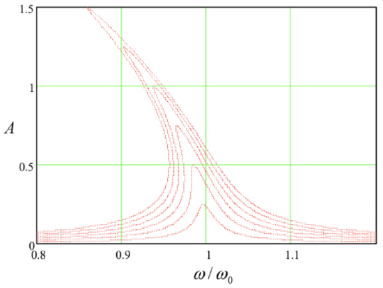
Figure 5.4. The nonlinear resonance in the Duffing oscillator, as described by Eq. (48), for the particular case α=ω20/6,δ/ω=0.01 (i.e. Q=50 ), and several values of the parameter f0/ω02, increased by equal steps of 0.005 from 0 to 0.03.
The same Eq. (50) also enables an estimate of the range of validity of our first approximation: since it has been based on the assumption |q(1)|<<|q(0)|≤A, for this particular problem we have to require αA2/32ω2<<1. For a pendulum (i.e. for α=ω20/6 ), this condition becomes A2<<192. Though numerical coefficients in such strong inequalities should be taken with a grain of salt, the large magnitude of this particular coefficient gives a good hint that the method may give very accurate results even for relatively large oscillations with A∼1. In Sec. 7 below, we will see that this is indeed the case.
From the mathematical viewpoint, the next step would be to write the next approximation as q(t)=AcosΨ+q(1)(t)+q(2)(t),q(2)∼ε2, and plug it into the Duffing equation (43), which (thanks to our special choice of q(0) and q(1) ) would retain only the sum ¨q(2)+ω2q(2) on its left-hand side. Again, requiring the amplitudes of two quadrature components of the frequency ω on the right-hand side to vanish, we may get second-order corrections to A and φ. Then we may use the remaining part of the equation to calculate q(2), and then go after the third-order terms, etc. However, for most purposes, the sum q(0)+q(1), and sometimes even just the crudest approximation q(0) alone, are completely sufficient. For example, according to Eq. (50), for a simple pendulum swinging as much as between the opposite horizontal positions (A=π/2), the 1st order correction q(1) is of the order of 0.5%. (Soon beyond this value, completely new dynamic phenomena start − see Sec. 7 below − but they cannot be described by these successive approximations at all.) Due to such reasons, higher approximations are rarely pursued for particular systems.
15 The same flexible approach is necessary to approximations used in quantum mechanics. The method discussed here is much closer in spirit (though not completely identical) to the WKB approximation (see, e.g., QM Sec. 2.4) rather than most perturbative approaches (QM Ch. 6).
16 The basic idea of this approach was reportedly suggested in 1920 by Balthasar van der Pol, and its first approximation (on which I will focus) is frequently called the van der Pol method. However, in optics and quantum mechanics, it is most commonly called the Rotating Wave Approximation (RWA). In math-oriented texts, this approach, especially its extensions to higher approximations, is usually called either the small parameter method or the asymptotic method. The list of other scientists credited for the development of this method, its variations, and extensions includes, most notably, N. Krylov, N. Bogolyubov, and Yu. Mitroplolsky.
17 This equation is frequently called the Duffing equation (or the equation of the Duffing oscillator), after Georg Duffing who carried out its first (rather incomplete) analysis in 1918.
18 For a mathematically rigorous treatment of higher approximations, see, e.g., Yu. Mitropolsky and N. Dao, Applied Asymptotic Methods in Nonlinear Oscillations, Springer, 2004. A more laymen (and, by today’s standards, somewhat verbose) discussion of various oscillatory phenomena may be found in the classical text A. Andronov, A. Vitt, and S. Khaikin, Theory of Oscillators, Dover, 2011.
19 Using the second of Eqs. (44), cosωt may be rewritten as cos(Ψ+φ)≡cosΨcosφ−sinΨsinφ. Then using the identity given, for example, by MA Eq. (3.4): cos3Ψ=(3/4)cosΨ+(1/4)cos3Ψ, we get Eq. (46).
20 The effect of pendulum’s frequency dependence on its oscillation amplitude was observed as early as 1673 by Christiaan Huygens - who by the way had invented the pendulum clock, increasing the timekeeping accuracy by about three orders of magnitude (and also discovered the largest of Saturn’s moons, Titan).