
10.3: Application of the Boundary Conditions to a Plane Interface


- Last updated
- Jun 21, 2021
- Save as PDF

( \newcommand{\kernel}{\mathrm{null}\,}\)
Returning to the problem of a wave incident on a plane interface as shown in Figure (10.1.1), one could satisfy the boundary condition on vecE by choosing the amplitude of the wave transmitted into the right half-space to be A= E0 for z=0, where E0 is the amplitude of the incident wave. This choice would, however, produce a discontinuity in Hy at the boundary because the ratio of Hy/Ex is different in the region z0. In order to match both Ex and Hy inside and outside the boundary it is necessary to assume that the oscillating dipoles in the material to the right of z=0 give rise to a reflected wave, so that for z<0, in the vacuum in this example, one has
Ex=E0exp(i[kz−ωt])+ERexp(−i[kz+ωt]),
and, since
Hy=1iωμ0∂Ex∂z,
Hy=√ϵ0μ0(E0exp(i[kz−ωt])−ERexp(−i[kz+ωt])),
where k = ω/c. In Equation (???) ER is the amplitude of the reflected wave, as yet undetermined. Notice the change in sign of the space part of the reflected wave phasor; this sign change is required because the reflected wave must propagate towards the left i.e. towards z=−∞. The expression for the magnetic field Hy is obtained from applying Maxwell’s equation (10.1.3) to Equation (???). From Equations (???) and (???) one obtains on the vacuum side of the interface at z=0
Ex(0)=(E0+ER)exp(−iωt)Hy(0)=√ϵ0μ0(E0−ER)exp(−iωt).
On the material side of the interface at z=0 one has
Ex(0)=Aexp(−iωt)Hy(0)=√ϵ0μ0(n+iκ)Aexp(−iωt).
Apply the boundary conditions that Ex and Hy must be continuous through the boundary at z=0 to obtain
E0+ER=A
and
E0−ER=(n+iκ)A.
These two equations can be readily solved:
T=AE0=2(1+n+iκ),R=ERE0=(1−(n+iκ)1+(n+iκ)).
Optical parameters n and κ are listed in Table(10.3.1) for green light and for a number of common materials. Metals are quite opaque at optical frequencies as can be seen from the Table. For example, at a wavelength of 0.5145 microns ( a standard Argon ion laser line) the optical electric field amplitude in copper falls to 1/e of its initial value in a distance δ = λ/2πκ, or δ = λ/16.3 = 31.5 × 10⁻⁹ meters. The attenuation of the fields in glass or in water at frequencies corresponding to visible light is very small, see Table(10.1). The attenuation coefficient, proportional to κ, is extremely sensitive to the presence of small amounts of impurities. Very pure glasses have been developed for use in optical fibres in which the length over which the field amplitudes have decayed by e−1 is in excess of 1 km.
It is of interest to calculate the absorption coefficient associated with the plane interface of Figure (10.1.1). This is the time-averaged rate at which energy flows into the surface divided by the time-averaged rate at which the incident wave carries power towards the surface. It can be calculated in two ways:
(1) As the difference between the time-averaged Poynting vectors for the incident and reflected waves divided by the incident wave Poynting vector. For the incident wave
<Sz0>=E202μ0c=E202Z0.
For the reflected wave
<Szr>=E2R2Z0.
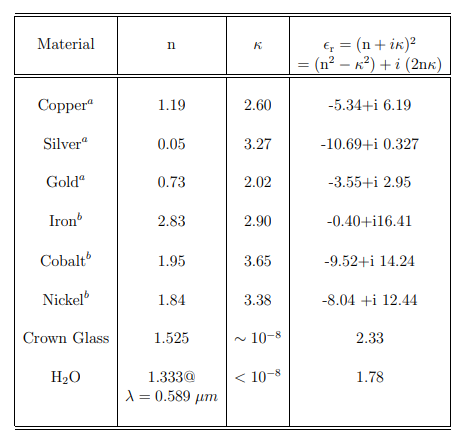
Table 10.3.1: Optical constants for some selected materials at a wavelength of 0.5145 microns ( 514.5 nm). This wavelength is a standard Argon ion laser green line. It corresponds to a frequency of f= 5.827 × 10¹⁴ Hz. A time dependence exp (−iωt) has been assumed. (a) P.B. Johnson and R.W. Christy, Phys.Rev.B6, 4370 (1972). (b) P.B. Johnson and R.W. Christy, Phys.Rev.B9, 5056 (1974).
In these last two equations Z0=√μ0/ϵ0=377 Ohms is the impedance of free space. Therefore, the absorption coefficient is given by
α=(<Sz0>−<Szr>)<Sz0>=1−|ERE0|2,
or, using Equation (10.3.10) for the reflection coefficient
α=4n(1+n)2+κ2,
(2) From the ratio of the time averaged Poynting vector just inside the material at z=0 to the incident wave Poynting vector.
<Sz>=12Real(H∗yEx)
<Sz>=12Real(√ϵ0μ0(n−iκ)A2)=n|A2|2Z0.
But from Equation (10.3.10)
|A2|=4E20(1+n)2+κ2,
and therefore the absorption coefficient is given by the same expression as was obtained above
α=<Sz><Sz0>=4n(1+n)2+κ2.