9.2: Waves incident on planar boundaries at angles

Introduction to waves propagating at angles

To determine electromagnetic fields we can generally solve a boundary value problem using the method of Section 9.1.1, the first step of which involves characterization of the basic quasistatic or dynamic fields and waves that could potentially exist within each separate region of the problem. The final solution is a linear combination of these basic fields and waves that matches all boundary conditions at the interfaces between the various regions.

So far we have considered only waves propagating along boundaries or normal to them. The general case involves waves incident upon boundaries at arbitrary angles, so we seek a compact notation characterizing such waves that simplifies the boundary value equations and their solutions. Because wave behavior at boundaries often becomes frequency dependent, it is convenient to use complex notation as introduced in Section 2.3.2 and reviewed in Appendix B, which can explicitly represent the frequency dependence of wave phenomena. For example, we might represent the electric field associated with a uniform plane wave propagating in the +z direction as \(\overline{\mathrm{\underline E}}_{\mathrm{o}} \mathrm{e}^{-\mathrm{j} \mathrm{kz}}\), where:

\[\overline{\mathrm{\underline E}}(\mathrm{z})=\overline{\mathrm{\underline E}}_{0} \mathrm{e}^{-\mathrm{j} \mathrm{k} \mathrm{z}}=\overline{\mathrm{\underline E}}_{0} \mathrm{e}^{-\mathrm{j} 2 \pi \mathrm{z} / \lambda} \label{9.2.1}\]

\[\overline{\mathrm{\underline E}}_{\mathrm{o}}=\hat{x} \underline{\mathrm{E}}_{\mathrm{ox}}+\hat{y} \underline{\mathrm{E}}_{\mathrm{oy}}\]

This notation is simpler than the time domain representation. For example, if this wave were x-polarized, then the compact complex notation \(\hat{x} \underline{\mathrm{E}}_{\mathrm{x}}\) would be replaced in the time domain by:

\[\begin{align}\overline{\mathrm{E}}(\mathrm{t}) &=\mathrm{R}_{\mathrm{e}}\left\{\hat{x} \underline{\mathrm{E}}_{\mathrm{x}}(\mathrm{z}) \mathrm{e}^{\mathrm{j} \omega \mathrm{t}}\right\}=\hat{x} \mathrm{R}_{\mathrm{e}}\left\{\left(\mathrm{R}_{\mathrm{e}}\left[\underline{\mathrm{E}}_{\mathrm{x}}(\mathrm{z})\right]+\mathrm{j} \mathrm{I}_{\mathrm{m}}\left[\underline{\mathrm{E}}_{\mathrm{x}}(\mathrm{z})\right]\right)(\cos \omega \mathrm{t}+\mathrm{j} \sin \omega \mathrm{t})\right\} \nonumber\\&=\hat{x}\left\{\mathrm{R}_{\mathrm{e}}\left[\underline{\mathrm{E}}_{\mathrm{x}}(\mathrm{z})\right] \cos \omega \mathrm{t}-\mathrm{I}_{\mathrm{m}}\left[\mathrm{\underline E}_{\mathrm{x}}(\mathrm{z})\right] \sin \omega \mathrm{t}\right\}\end{align}\]

The more general time-domain expression including both x and y components would be twice as long. Thus complex notation adequately characterizes frequency-dependent wave propagation and is more compact.

The physical significance of Equation \ref{9.2.1} is divided into two parts: \(\mathrm{\overline{\underline E}_{0}}\) tells us the polarization, amplitude, and absolute phase of the wave at the origin, and \(\mathrm{e}^{-\mathrm{j} 2 \pi z / \lambda} \equiv \mathrm{e}^{\mathrm{j} \phi(z)}\) tells us how the phase φ of this wave varies with position. In this case the phase decreases 2\(\pi\) radians as z increases by one wavelength λ. The physical significance of a phase shift φ of -2\(\pi\) radians for z = λ is that observers located at z = λ experience a delay of 2\(\pi\) radians; for pure sinusoids a phase shift of 2\(\pi\) is of course not observable.

Waves propagating in arbitrary directions are therefore easily represented by expressions similar to Equation \ref{9.2.1}, but with a phase φ that is a function of x, y, and z. For example, a general plane wave would be:

\[\overline{\mathrm{\underline E}}(\mathrm{z})=\overline{\mathrm{\underline E}}_{0} \mathrm{e}^{-\mathrm{j} \mathrm{k}_{\mathrm{x}} \mathrm{x}-\mathrm{j} \mathrm{k}_{\mathrm{y}} \mathrm{y}-\mathrm{jk}_{\mathrm{z}} \mathrm{z}}=\underline{\mathrm{\overline E}}_{\mathrm{o}} \mathrm{e}^{-\mathrm{j} \overline{\mathrm{k}} \cdot \mathrm{\overline r}}\]

where \( \overline{\mathrm{r}}=\hat{x} \mathrm{x}+\hat{y} \mathrm{y}+\hat{z} \mathrm{z}\) and:

\[\overline{\mathrm{k}}=\hat{\mathrm{x}} \mathrm{k}_{\mathrm{x}}+\hat{\mathrm{y}} \mathrm{k}_{\mathrm{y}}+\hat{\mathrm{z}} \mathrm{k}_{\mathrm{z}}\]

We call \(\overline k\) the propagation vector or wave number \(\overline k\). The wave numbers k_x, k_y, and k_z have the dimensions of radians per meter and determine how rapidly the wave phase φ varies with position along the x, y, and z axes, respectively. Positions having the same value for \(\overline{\mathrm{k}} \bullet \overline{\mathrm{r}}\) have the same phase and are located on the same phase front. A wave with a planar phase fronts is a plane wave, and if its amplitude is constant across any phase front, it is a uniform plane wave.

Figure \(\PageIndex{1}\): Uniform plane wave propagating at angle θ in the x-z plane.

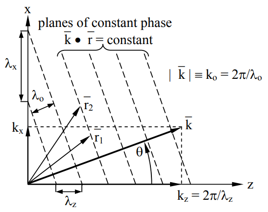
The vector \(\overline k\) points in the direction of propagation for uniform plane waves. The geometry is represented in Figure 9.2.1 for a uniform plane wave propagating in the x-z plane at an angle θ and wavelength λ_o. The planes of constant phase are perpendicular to the wave vector \(\overline k\) because \(\overline{\mathrm{k}} \bullet \overline{\mathrm{r}}\) must be constant everywhere in such a plane.

The solution (9.2.4) can be substituted into the wave equation (2.3.21):

\[\left(\nabla^{2}+\omega^{2} \mu \varepsilon\right) \overline{\mathrm{\underline E}}=0\]

This substitution yields⁴⁷:

\[\left[-\left(k_{x}^{2}+k_{y}^{2}+k_{z}^{2}\right)+\omega^{2} \mu \varepsilon\right] \overline{\underline {\mathrm E}}=0\]

\[\mathrm{k}_{\mathrm{x}}^{2}+\mathrm{k}_{\mathrm{y}}^{2}+\mathrm{k}_{\mathrm{z}}^{2}=\mathrm{k}_{\mathrm{o}}^{2}=\omega^{2} \mu \varepsilon=|\overline{\mathrm{k}}|^{2}=\overline{\mathrm{k}} \bullet \overline{\mathrm{k}}\]

⁴⁷ \(\nabla^{2} \underline{\mathrm{\overline E}}=\left(\partial^{2} / \partial \mathrm{x}^{2}+\partial^{2} / \partial \mathrm{y}^{2}+\partial^{2} / \partial \mathrm{z}^{2}\right) \overline{\mathrm{\underline E}}=-\left(\mathrm{k}_{\mathrm{x}}^{2}+\mathrm{k}_{\mathrm{y}}^{2}+\mathrm{k}_{\mathrm{z}}^{2}\right) \overline{\mathrm{\underline E}}\).

Therefore the figure and (9.2.7) suggest that:

\[\mathrm{k}_{\mathrm{x}}=\overline{\mathrm{k}} \bullet \hat{x}=\mathrm{k}_{\mathrm{o}} \sin \theta, \mathrm{k}_{\mathrm{z}}=\overline{\mathrm{k}} \bullet \hat{z}=\mathrm{k}_{\mathrm{o}} \cos \theta\]

The figure also includes the wave propagation vector components \( \hat{x} \mathrm{k}_{\mathrm{x}}\) and \( \hat{z} \mathrm{k}_{\mathrm{z}}\).

Three projected wavelengths, λ_x, λ_y, and λ_z, are perceived by observers moving along those three axes. The distance between successive wavefronts at 2\(\pi\) phase intervals is λ_o in the direction of propagation, and the distances separating these same wavefronts as measured along the x and z axes are equal or greater, as illustrated in Figure 9.2.1. For example:

\[\lambda_{\mathrm{z}}=\lambda_{\mathrm{o}} / \cos \theta=2 \pi / \mathrm{k}_{\mathrm{z}} \geq \lambda_{\mathrm{o}}\]

Combining (9.2.8) and (9.2.10) yields:

\[\lambda_{\mathrm{x}}^{-2}+\lambda_{\mathrm{y}}^{-2}+\lambda_{\mathrm{z}}^{-2}=\lambda_{\mathrm{o}}^{-2}\]

The electric field \( \overline{\mathrm{\underline E}}(\overline{\mathrm{r}})\) for the wave of Figure 9.2.1 propagating in the x-z plane is orthogonal to the wave propagation vector \(\overline{\mathrm{k}} \). For simplicity we assume this wave is ypolarized:

\[\overline{\mathrm{\underline E}}(\overline{\mathrm{r}})=\hat{y} \underline{\mathrm{E}}_{0} \mathrm{e}^{-\mathrm{j} \overline{\mathrm{k}} \cdot \mathrm{\overline r}}\]

The corresponding magnetic field is:

\[\begin{align}\overline{\mathrm{\underline H}}(\overline{\mathrm{r}}) &=-(\nabla \times \overline{\mathrm{\underline E}}) / \mathrm{\mathrm{j} \omega \mu_{\mathrm{o}}=\left(\hat{x} \partial \mathrm{E}_{\mathrm{y}} / \partial \mathrm{z}-\hat{z} \partial \mathrm{\underline E}_{\mathrm{y}} / \partial \mathrm{x}\right) / \mathrm{j} \omega \mu_{\mathrm{o}}} \nonumber\\&=(\hat{z} \sin \theta-\hat{x} \cos \theta)\left(\mathrm{E}_{\mathrm{o}} / \eta_{\mathrm{o}}\right) \mathrm{e}^{-\mathrm{j} \mathrm{\overline k} \cdot \mathrm{\overline r}}\end{align}\]

One difference between this uniform y-polarized plane wave propagating at an angle and one propagating along a cartesian axis is that \(\overline{\mathrm{H}}\) no longer lies along a single axis, although it remains perpendicular to both \(\overline{\mathrm{E}}\) and \(\overline{\mathrm{k}}\). The next section treats such waves further.

Example \(\PageIndex{A}\)

If λ_x = 2λ_z in Figure 9.2.1, what are θ, λ_o, and \(\overline{\mathrm{k}}\)?

Solution

By geometry, \(\theta=\tan ^{-1}\left(\lambda_{z} / \lambda_{x}\right)=\tan ^{-1} 0.5 \cong 27^{\circ}\). By (9.2.11) \(\lambda_{\mathrm{o}}^{-2}=\lambda_{\mathrm{x}}^{-2}+\lambda_{\mathrm{z}}^{-2}=(0.25+1) \lambda_{\mathrm{Z}}^{-2}\), so \(\lambda_{\mathrm{o}}=1.25^{-0.5} \lambda_{\mathrm{z}}=0.89 \lambda_{\mathrm{z}}\). \(\overline{\mathrm{k}}=\hat{x} \mathrm{k}_{\mathrm{x}}+\hat{z} \mathrm{k}_{\mathrm{z}}=\hat{x} \mathrm{k}_{\mathrm{o}} \sin \theta+\hat{z} \mathrm{k}_{\mathrm{o}} \cos \theta\), where \(\mathrm{k}_{\mathrm{o}}=2 \pi / \lambda_{\mathrm{o}}\). Alternatively, \(\overline{\mathrm{k}}=\hat{x} 2 \pi / \lambda_{\mathrm{x}}+\hat{z} 2 \pi / \lambda_{\mathrm{z}}\).

Waves at planar dielectric boundaries

Waves at planar dielectric boundaries are solved using the boundary-value-problem method of Section 9.1.4 applied to waves propagating at angles, as introduced in Section 9.2.1.

Because the behavior of waves at an interface depends upon their polarization we need a coordinate system for characterizing it. For this purpose the plane of incidence is defined as the plane of projection of the incident wave propagation vector \(\overline{\mathrm{k}}\) upon the interface, as illustrated in Figure 9.2.2(a). One cartesian axis is traditionally defined as being normal to this plane of incidence; in the figure it is the y axis.

Figure \(\PageIndex{2}\): Uniform plane wave incident upon a planar interface.

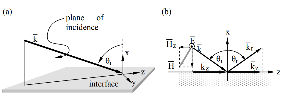
We know from Section 2.3.4 that any pair of orthogonally polarized uniform plane waves can be superimposed to achieve any arbitrary wave polarization. For example, x- and ypolarized waves can be superimposed. It is customary to recognize two simple types of incident electromagnetic waves that can be superimposed to yield any incident wave polarization: transverse electric waves (TE waves) are linearly polarized transverse to the plane of incidence (y-polarized in the figure), and transverse magnetic waves (TM waves) have the orthogonal linear polarization so that the magnetic field is purely transverse (again if y-polarized). TE and TM waves are typically transmitted and reflected with different amplitudes.

Consider first a TE wave incident upon the planar interface of Figure 9.2.2(b) at the incidence angle θ_i. The corresponding \( \overline{\mathrm{H}}\) lies in the x-z plane and is orthogonal to \( \overline{\mathrm{E}}\). \(\overline{\mathrm{H}} \) points downward in the figure, corresponding to power \(\overline{\mathrm{S}}=\overline{\mathrm{E}} \times \overline{\mathrm{H}} \) propagating toward the interface, where \( \overline{\mathrm{S}}\) is the Poynting vector for the incident wave. The wavelength of the wave above the interface is \(\lambda_{\mathrm{o}}=1 /(\mathrm{f} \sqrt{\mu \varepsilon}) \) in the medium characterized by permittivity ε and permeability μ. The medium into which the wave is partially transmitted is characterized by ε_t and μ_t, and there the wave has wavelength \( \lambda_{\mathrm{t}}=1 /(\mathrm{f} \sqrt{\mu_{\mathrm{t}} \varepsilon_{\mathrm{t}}})\) and the same frequency f. This incident TE wave can be characterized by:

\[\overline{\mathrm{\underline E}}_{\mathrm{i}}=\hat{y} \mathrm{\underline E}_{\mathrm{o}} \mathrm{e}^{\mathrm{j} \mathrm{k}_{\mathrm{x}} \mathrm{x}-\mathrm{j} \mathrm{k}_\mathrm{z} \mathrm{z}}\ \left[\mathrm{Vm}^{-1}\right]\]

\[\overline{\mathrm{\underline H}}_{\mathrm{i}}=-\left(\underline{\mathrm{E}}_{\mathrm{o}} / \eta\right)\left(\hat{x} \sin \theta_{\mathrm{i}}+\hat{z} \cos \theta_{\mathrm{i}}\right) \mathrm{e}^{\mathrm{j} \mathrm{k}_{\mathrm{x}} \mathrm{x}-\mathrm{j} \mathrm{k}_{\mathrm{z}} \mathrm{z} } \ \left[\mathrm{Am}^{-1}\right]\]

where the characteristic impedance of the incident medium is \( \eta=\sqrt{\mu / \varepsilon}\), and \(\overline{\mathrm{H}} \) is orthogonal to \(\overline{\mathrm{E}} \).

The transmitted wave would generally be similar, but with a different η_t, θ_t, E_t, and \(\overline{\mathrm{k}}_{\mathrm t}\). We might expect a reflected wave as well. The boundary-value-problem method of Section 9.1.2 requires expressions for all waves that might be present in both regions of this problem. In addition to the incident wave we therefore might add general expressions for reflected and transmitted waves having the same TE polarization. If still other waves were needed then no solution satisfying all Maxwell’s equations would emerge until they were added too; we shall see no others are needed here. These general reflected and transmitted waves are:

\[\overline{\mathrm{\underline E}}_{\mathrm{r}}=\hat{y} \underline{\mathrm{E}}_{\mathrm{r}} \mathrm{e}^{-\mathrm{j} \mathrm{k}_{\mathrm{rx}} \mathrm{x}-\mathrm{j} \mathrm{k}_{\mathrm{rz}} \mathrm{z}} \ \left[\mathrm{Vm}^{-1}\right]\]

\[\overline{\mathrm{\underline H}}_{\mathrm{r}}=\left(\underline{\mathrm{E}}_{\mathrm{r}} / \eta\right)\left(-\hat{x} \sin \theta_{\mathrm{r}}+\hat{z} \cos \theta_{\mathrm{r}}\right) \mathrm{e}^{-\mathrm{j} \mathrm{k}_{\mathrm{rx}} \mathrm{x}-\mathrm{j} \mathrm{k}_{\mathrm{rz}} \mathrm{z}} \ \left[\mathrm{Am}^{-1}\right]\]

\[\overline{\mathrm{\underline E}}_{\mathrm{t}}=\hat{y} \mathrm{\underline E}_{\mathrm{t}} \mathrm{e}^{\mathrm{jk}_{\mathrm{tx}} \mathrm{x}-\mathrm{jk}_{\mathrm{tz}} \mathrm{z}} \ \left[\mathrm{Vm}^{-1}\right]\]

\[\overline{\mathrm{\underline H}}_{\mathrm{t}}=-\left(\mathrm{\underline E}_{\mathrm{t}} / \eta_{\mathrm{t}}\right)\left(\hat{x} \sin \theta_{\mathrm{t}}+\hat{z} \cos \theta_{\mathrm{t}}\right) \mathrm{e}^{\mathrm{jk}_{\mathrm{tx}} \mathrm{x}-\mathrm{j} \mathrm{k}_{\mathrm{tz}} \mathrm{z}} \ \left[\mathrm{Am}^{-1}\right]\]

Boundary conditions that must be met everywhere on the non-conducting surface at x = 0 include:

\[\overline{\mathrm{\underline E}}_{\mathrm{i} / /}+\overline{\mathrm{\underline E}}_{\mathrm{r} / /}=\overline{\mathrm{\underline E}}_{\mathrm{t} / /}\]

\[\overline{\mathrm{\underline H}}_{\mathrm{i} / /}+\overline{\mathrm{\underline H}}_{\mathrm{r} / /}=\overline{\mathrm{\underline H}}_{\mathrm{t} / /}\]

Substituting into (9.2.20) the values of \(\overline{\mathrm{\underline E}}_{/ /} \) at the boundaries yields:

\[\underline{E}_{0} \mathrm{e}^{-j \mathrm{k}_{\mathrm{z}} \mathrm{z}}+\underline{\mathrm{E}}_{\mathrm{r}} \mathrm{e}^{-\mathrm{j} \mathrm{k}_{\mathrm{rz}} \mathrm{z}}=\underline{\mathrm{E}}_{\mathrm{t}} \mathrm{e}^{-\mathrm{j} \mathrm{k}_{\mathrm{t} \mathrm{z}} {\mathrm{z}}}\]

This equation can be satisfied for all values of z only if all exponents are equal. Therefore e^−jk_zz can be factored out, simplifying the boundary-condition equations for both \(\overline{\mathrm{\underline E}}_{/ /} \) and \(\overline{\mathrm{\underline H}}_{/ /} \).

\[\mathrm{\underline{E}_{0}+\underline{E}_{r}=\underline{E}_{t}} \qquad \qquad \qquad \text{(boundary condition for } \mathrm{E}_{//})\]

\[\mathrm{\frac{\underline E_{0}}{\eta} \cos \theta_{i}-\frac{\underline E_{r}}{\eta} \cos \theta_{r}=\frac{\underline E_{t}}{\eta_{t}} \cos \theta_{t}} \qquad \qquad \qquad \text{(boundary condition for } \mathrm{H}_{//})\]

Because the exponential terms in (9.2.22) are all equal, it follows that the phases of all three waves must match along the full boundary, and:

\[\mathrm{k}_{\mathrm{iz}}=\mathrm{k}_{\mathrm{rz}}=\mathrm{k}_{\mathrm{tz}}=\mathrm{k}_{\mathrm{i}} \sin \theta_{\mathrm{i}}=\mathrm{k}_{\mathrm{i}} \sin \theta_{\mathrm{r}}=\mathrm{k}_{\mathrm{t}} \sin \theta_{\mathrm{t}}=2 \pi / \lambda_{\mathrm{z}}\]

This phase-matching condition implies that the wavelengths of all three waves in the z direction must equal the same λ_z. It also implies that the angle of reflection θ_r equals the angle of incidence θ_i, and that the angle of transmission θ_t is related to θ_i by Snell’s law:

\[\frac{\sin \theta_{\mathrm{t}}}{\sin \theta_{\mathrm{i}}}=\frac{\mathrm{k}_{\mathrm{i}}}{\mathrm{k}_{\mathrm{t}}}=\frac{\mathrm{c}_{\mathrm{t}}}{\mathrm{c}_{\mathrm{i}}}=\sqrt{\frac{\mu \varepsilon}{\mu_{\mathrm{t}} \varepsilon_{\mathrm{t}}}} \qquad \qquad \qquad \text{(Snell’s law)}\]

If μ = μ_t, then the angle of transmission becomes:

\[\theta_{\mathrm{t}}=\sin ^{-1}\left(\sin \theta_{\mathrm{i}} \sqrt{\frac{\varepsilon}{\varepsilon_{\mathrm{t}}}}\right)\]

These phase-matching constraints, including Snell’s law, apply equally to TM waves.

The magnitudes of the reflected and transmitted TE waves can be found by solving the simultaneous equations (9.2.23) and (9.2.24):

\[\mathrm{\underline{E}_{r} / \underline{E}_{0}=\underline{\Gamma}\left(\theta_{i}\right)=\frac{\eta_{t} \cos \theta_{i}-\eta \cos \theta_{t}}{\eta_{t} \cos \theta_{i}+\eta \cos \theta_{t}}=\frac{\eta_{n}^{\prime}-1}{\eta_{n}^{\prime}+1}}\]

\[\mathrm{\underline E}_{\mathrm{t}} / \mathrm{\underline E}_{\mathrm{o}}=\mathrm{\underline T}\left(\theta_{\mathrm{i}}\right)=\frac{2 \eta_{\mathrm{t}} \cos \theta_{\mathrm{i}}}{\eta_{\mathrm{t}} \cos \theta_{\mathrm{i}}+\eta \cos \theta_{\mathrm{t}}}=\frac{2 \eta_{\mathrm{n}}^{\prime}}{\eta_{\mathrm{n}}^{\prime}+1}\]

where we have defined the normalized angular impedance for TE waves as \(\eta_{\mathrm{n}}^{\prime} \equiv \eta_{\mathrm{t}} \cos \theta_{\mathrm{i}} /\left(\eta \cos \theta_{\mathrm{t}}\right)\). The complex angular reflection and transmission coefficients \(\underline{\Gamma}\) and \(\underline T\) for TE waves approach those given by (9.1.19) and (9.1.20) for normal incidence in the limit θ_i → 0. The limit of grazing incidence is not so simple, and even the form of the transmitted wave can change markedly if it becomes evanescent, as discussed in the next section. The results for incident TM waves are postponed to Section 9.2.6. Figure 9.2.6(a) plots \(|\underline\Gamma(\theta)|^{2}\) for a typical dielectric interface. It is sometimes useful to note that (9.2.28) and (9.2.29) also apply to equivalent TEM lines for which the characteristic impedances of the input and output lines are \(\eta_{i} / \cos \theta_{i} \) and \(\eta_{t} / \cos \theta_{t} \), respectively. When TM waves are incident, the corresponding equivalent impedances are \( \eta_{\mathrm{i}} \cos \theta_{\mathrm{i}}\) and \(\eta_{\mathrm{t}} \cos \theta_{\mathrm{t}}\), respectively.

Example \(\PageIndex{B}\)

What fraction of the normally incident power (θ_i = 0) is reflected by a single glass camera lense having ε = 2.25ε_o? If θ_i = 30^o , what is θ_t in the glass?

Solution

At each interface between air and glass, (9.2.28) yields for θ_i = 0: \(\underline \Gamma_{L}=\left(\eta_{\mathrm{n}}^{\prime}-1\right) /\left(\eta_{\mathrm{n}}^{\prime}+1\right)\), where \(\eta_{\mathrm{n}}^{\prime}=\left(\eta_{\mathrm{glass}} \cos \theta_{\mathrm{i}}\right) /\left(\eta_{\mathrm{air}} \cos \theta_{\mathrm{t}}\right)=\left(\varepsilon_{\mathrm{i}} / \varepsilon_{\mathrm{g}}\right)^{0.5}=1 / 1.5\). Thus \(\underline \Gamma_{L}=(1- 1.5)/(1 + 1.5) = -0.2\), and \(|\underline\Gamma|^{2}=0.04\), so ~4 percent of the power is reflected from each of the two curved surfaces for each independent lense, or ~8 percent total; these reflections are incoherent so their reflected powers add. Modern lenses have many elements with different permittivities, but coatings on them reduce these reflections, as discussed in Section 7.3.2 for quarter-wave transformers. Snell’s law (9.2.26) yields \(\theta_{t}=\sin ^{-1}\left[\left(\varepsilon_{i} / \varepsilon_{t}\right)^{0.5} \sin \theta_{i}\right]=\sin ^{-1}[(1 / 1.5)(0.5)]=19.5^{\circ}\).

Evanescent waves

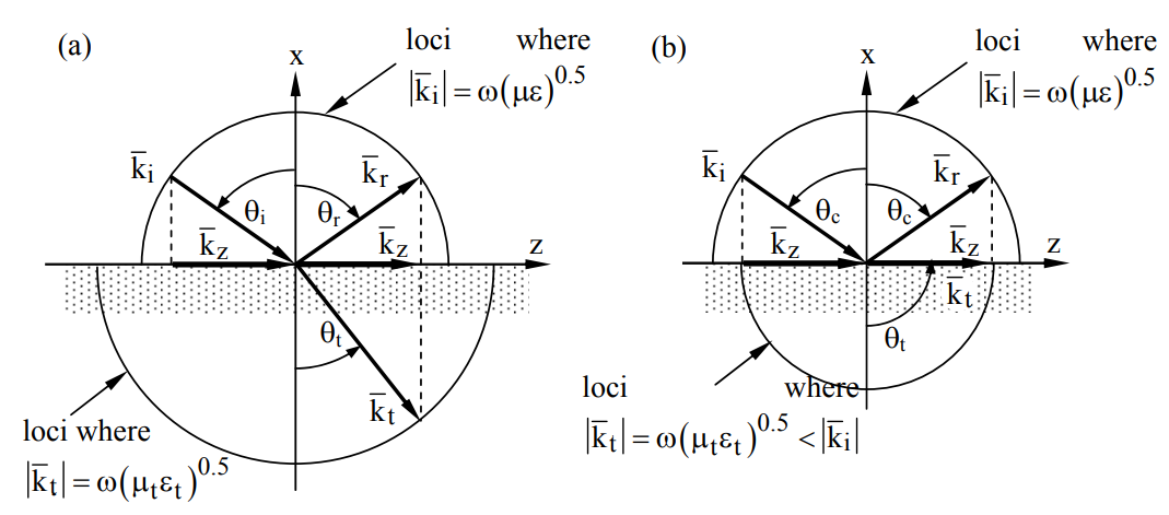
Figure 9.2.3 suggests why a special form of electromagnetic wave is sometimes required in order to satisfy boundary conditions. Figure 9.2.3(a) illustrates how the required equality of the z components of the incident, reflected, and transmitted wave propagation vectors \(\overline{\mathrm{k}}\) controls the angles of reflection and transmission, θ_r and θ_t. The radii of the two semi-circles correspond to the magnitudes of \(\overline{\mathrm{k}}_{\mathrm i}\) and \(\overline{\mathrm{k}}_{\mathrm t}\).

Figure 9.2.3(b) shows that a wave incident at a certain critical angle θ_c will produce a transmitted wave propagating parallel to the interface, provided \(\left|\overline{\mathrm{k}}_{\mathrm{t}}\right|<\left|\overline{\mathrm{k}}_{\mathrm{i}}\right|\). Snell’s law (9.2.26) can be evaluated for sin θ_t = 1 to yield:

\[\theta_{\mathrm{c}}=\sin ^{-1}\left(\mathrm{c}_{\mathrm{i}} / \mathrm{c}_{\mathrm{t}}\right) \text { for } \mathrm{c}_{\mathrm{i}}<\mathrm{c}_{\mathrm{t}} \qquad\qquad\qquad \text { (critical angle) }\]

Figures 9.2.3(b) illustrates why phase matching is impossible with uniform plane waves when θ> θ_c; \(\mathrm{k}_{\mathrm{z}}>\left|\overline{\mathrm{k}}_{\mathrm{t}}\right|\). Therefore the λ_z determined by λ and θ_i is less than λ_t, the natural wavelength of the transmission medium at frequency ω. A non-uniform plane wave is then required for phase matching, as discussed below.

Figure \(\PageIndex{3}\): Angles of reflection and transmission, and the critical angle θ_c.

The wave propagation vector \( \overline{\mathrm{k}}_{\mathrm{t}}\) must satisfy the wave equation \(\left(\nabla^{2}+\mathrm{k}_{\mathrm{t}}^{2}\right) \overline{\mathrm{\underline E}}=0 \). Therefore the transmitted wave must be proportional to \(\mathrm{e}^{-\mathrm{j} \overline{\mathrm{k}}_\mathrm{t} \cdot \mathrm{\overline r}} \), where \(\overline{\mathrm{k}}_{\mathrm{t}}=\hat{k} \mathrm{k}_{\mathrm{t}} \) and k_z = k_i sin θ_i, satisfy the expression:

\[\mathrm{k}_{\mathrm{t}}^{2}=\omega^{2} \mu_{\mathrm{t}} \varepsilon_{\mathrm{t}}=\mathrm{k}_{\mathrm{tx}}^{2}+\mathrm{k}_{\mathrm{z}}^{2}\]

When \(\mathrm{k}_{\mathrm{t}}^{2}<\mathrm{k}_{\mathrm{z}}^{2} \) it follows that:

\[ \mathrm{k_{t x}=\pm j\left(k_{z}^{2}-k_{t}^{2}\right)^{0.5}=\pm j \alpha}\]

We choose the positive sign for \(\alpha\) so that the wave amplitude decays with distance from the power source rather than growing exponentially.

The transmitted wave then becomes:

\[\overline{\mathrm{\underline E}}_{\mathrm{t}}(\mathrm{x}, \mathrm{z})=\hat{y} \underline{\mathrm{E}}_{\mathrm{t}} \mathrm{e}^{\mathrm{j} \mathrm{k}_{\mathrm{tx}} \mathrm{x}-\mathrm{jk}_{\mathrm{z}} \mathrm{z}}=\hat{y} \mathrm{\underline E}_{\mathrm{t}} \mathrm{e}^{\alpha \mathrm{x}-\mathrm{j} \mathrm{k}_{\mathrm{z}}{\mathrm{z}}}\]

Note that x is negative in the decay region. The rate of decay \( \mathrm{\alpha=\left(k_{i}^{2} \sin ^{2} \theta_{i}-k_{t}^{2}\right)^{0.5}}\) is zero when θ_i = θ_c and increases as θ_i increases past θ_c; Waves that decay with distance from an interface and propagate power parallel to it are called surface waves.

The associated magnetic field \(\overline{\mathrm{\underline H}}_{\mathrm{t}}\) can be found by substituting (9.2.33) into Faraday’s law:

\[\overline{\mathrm{\underline H}}_{\mathrm{t}}=\nabla \times \overline{\mathrm{\underline E}} /\left(-\mathrm{j} \omega \mu_{\mathrm{t}}\right)=-\left(\underline{\mathrm{E}}_{\mathrm{t}} / \eta_{\mathrm{t}}\right)\left(\hat{x} \sin \theta_{\mathrm{t}}-\hat{\mathrm{z}} \cos \theta_{\mathrm{t}}\right) \mathrm{e}^{\alpha \mathrm{x}-\mathrm{j} \mathrm{k}_{\mathrm{z}} \mathrm{z}}\]

This is the same expression as (9.2.19), which was obtained for normal incidence, except that the magnetic field and wave now decay with distance x from the interface rather than propagating in that direction. Also, since sinθ_t > 1 for θ_i > θ_c, cosθ_t is now imaginary and positive, and \(\overline{\mathrm{H}}\) is not in phase with \( \overline{\mathrm{E}}\). As a result, Poynting’s vector for these surface waves has a real part corresponding to real power propagating parallel to the surface, and an imaginary part corresponding to reactive power flowing perpendicular to the surface in the direction of wave decay:

\[\overline{\mathrm{\underline S}}=\overline{\mathrm{\underline E}} \times \overline{\mathrm{\underline H}}^{*}=\left(-\mathrm{j} \alpha \hat{x}+\mathrm{k}_{\mathrm{z}} \hat{z}\right)\left(\left|\overline{\mathrm{\underline E}}_{\mathrm{t}}\right|^{2} / \omega \mu_{\mathrm{t}}\right) \mathrm{e}^{2 \alpha \mathrm{x}} \ \left[\mathrm{Wm}^{-2}\right]\]

The reactive part flowing in the \(-\hat{x} \) direction is \(\mathrm{+j \alpha\left|\underline{E}_{t}\right|^{2} / \omega \mu_{t} e^{2 a x}} \) and is therefore inductive (+j), corresponding to an excess of magnetic stored energy relative to electric energy within this surface wave. A wave such as this one that decays in a direction for which the power flow is purely reactive is designated an evanescent wave.

An instantaneous view of the electric and magnetic fields of a non-uniform TE plane wave formed at such a dielectric boundary is shown in Figure 9.2.4; these correspond to the fields of (9.2.33) and (9.2.34).

Figure \(\PageIndex{4}\): Evanescent wave traveling in the +z direction at a dielectric interface.

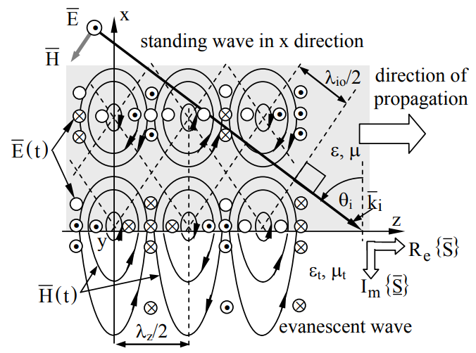
The conventional notation used here indicates field strength by the density of symbols or field lines, and the arrows indicate field direction. Small circles correspond to field lines pointing perpendicular to the page; center dots indicate field lines pointing out of the page in the +y direction and center crosses indicate the opposite, i.e., field lines pointing into the page.

The time average wave intensity in the \(+\hat{z} \) direction for x negative and outside the dielectric is:

\[\mathrm{P}_{\mathrm{z}}=0.5 \mathrm{R}_{\mathrm{e}}\left\{\overline{\mathrm{\underline E}} \times \overline{\mathrm{\underline H}}^{*}\right\}=\left(\mathrm{k}_{\mathrm{z}}\left|\mathrm{\underline E}_{\mathrm{t}}\right|^{2} / 2 \omega \mu_{\mathrm{t}}\right) \mathrm{e}^{\alpha \mathrm{x}} \ \left[\mathrm{W} \mathrm{m}^{-2}\right]\]

Since the real and imaginary parts of \(\underline{\mathrm{\overline S}} \) are orthogonal, there is no decay in the direction of propagation, and therefore no power absorption or heating of the media. Beyond the critical angle θ_c the power is perfectly reflected. In the next section we shall see that the real and imaginary parts of \(\underline{\mathrm{\overline S}} \) are often neither orthogonal nor parallel.

Waves in lossy media

Sometimes one or both of the two media are conductive. This section explores the nature of waves propagating in such lossy media having conductivity σ > 0. Section 9.2.5 then discusses reflections from such media. Losses can also arise if ε or μ are complex. The quasistatic relaxation of charge, current, and field distributions in lossy media is discussed separately in Section 4.3.

We can determine the nature of waves in lossy media using the approach of Section 2.3.3 and including the conduction currents \(\overline{\mathrm{J}} \) in Ampere’s law:

\[\nabla \times \overline{\mathrm{\underline H}}=\overline{\mathrm{\underline J}}+\mathrm{j} \omega \underline{\varepsilon} \overline{\mathrm{\underline E}}=\sigma \overline{\mathrm{\underline E}}+j \omega \underline{\varepsilon} \underline{\mathrm{\overline E}}=j \omega \underline{\varepsilon}_{\mathrm{eff}} \overline{\mathrm{\underline E}}\]

where the effective complex permittivity \( \underline{\varepsilon}_{\mathrm{eff}}\) is:

\[\underline{\varepsilon}_{\mathrm{eff}}=\varepsilon[1-(\mathrm{j} \sigma / \omega \varepsilon)]\]

The quantity σ/ωε is called the loss tangent of the medium and indicates how fast waves decay. As we shall see, waves propagate well if σ ωε, sometimes within a fraction of a wavelength.

Substituting \(\underline{\varepsilon}_{\mathrm{eff}}) for ε in k² = ω²με yields the dispersion relation:

\[\mathrm{\underline{k}^{2}=\omega^{2} \mu \varepsilon[1-(j \sigma / \omega \varepsilon)]=\left(k^{\prime}-j k^{\prime \prime}\right)^{2}}\]

where we define the complex wavenumber \(\underline{\mathrm{k}}\) in terms of its real and imaginary parts as:

\[\mathrm{\underline{k}=k^{\prime}-j k^{\prime \prime}}\]

The form of the wave solution, following (2.3.26), is therefore:

\[\overline{\mathrm{\underline E}}(\overline{\mathrm{r}})=\hat{y} \mathrm{E}_{\mathrm{o}} \mathrm{e}^{-\mathrm{j} \mathrm{k}^{\prime} \mathrm{z}-\mathrm{k}^{\prime \prime} \mathrm{z}} \ \left[\mathrm{v} \mathrm{m}^{-1}\right]\]

This wave has wavelength λ′, frequency ω, and phase velocity v_p inside the conductor related by:

\[\mathrm{k}^{\prime}=2 \pi / \lambda^{\prime}=\omega / \mathrm{v}_{\mathrm{p}}\]

and the wave decays exponentially with z as \( \mathrm{e}^{-\mathrm{k}^{\prime \prime} \mathrm{z}}=\mathrm{e}^{-\mathrm{z} / \Delta}\). Note that the wave decays in the same direction as it propagates, corresponding to power dissipation, and that the 1/e penetration depth Δ is 1/k" meters. Inside conductors, λ′ and v_p are much less than their free-space values.

We now need to determine k' and k". In general, matching the real and imaginary parts of (9.2.39) yields two equations that can be solved for k' and k":

\[\left(\mathrm{k}^{\prime}\right)^{2}-\left(\mathrm{k}^{\prime \prime}\right)^{2}=\omega^{2} \mu \varepsilon\]

\[2 \mathrm{k}^{\prime} \mathrm{k}^{\prime \prime}=\omega \mu \sigma\]

However, in the limits of very high or very low values of the loss tangent σ/ωε, it is much easier to evaluate (9.2.39) directly.

In the low loss limit where σ << ωε, (9.2.39) yields:

\[\underline{\mathrm{k}}=\omega \sqrt{\mu \varepsilon[1-(\mathrm{j} \sigma / \omega \varepsilon)]} \cong \omega \sqrt{\mu \varepsilon}-\mathrm{j} \sigma \eta / 2 \quad(\sigma<<\omega \varepsilon)\]

where the approximate wave impedance of the medium is \(\eta=\sqrt{\mu / \varepsilon}\), and we have used the Taylor series approximation \(\sqrt{1+\delta} \cong 1+\delta / 2\) for δ << 1. In this limit we see from (9.2.45) that λ′ and v_p ≅ c are approximately the same as they are for the lossless case, and that the 1/e penetration depth \(\Delta \cong 2 / \sigma \eta\), which becomes extremely large as σ → 0.

In the high loss limit where σ >> ωε, (9.2.39) yields:

\[\begin{align} \underline{\mathrm k} &=\mathrm{\omega \sqrt{\mu \varepsilon[1-(j \sigma / \omega \varepsilon)]} \cong \sqrt{-j \mu \omega \sigma}} \qquad(\sigma>>\omega \varepsilon) \\ & \mathrm{\cong \sqrt{\omega \mu \sigma} \sqrt{-j}=\pm \sqrt{\frac{\omega \mu \sigma}{2}}(1-j)} \end{align}\]

The real and imaginary parts of \(\underline{\mathrm{k}}\) have the same magnitudes, and the choice of sign determines the direction of propagation. The wave generally decays exponentially as it propagates, although exponential growth occurs in media with negative conductivity. The penetration depth is commonly called the skin depth δ in this limit (σ >> ωε), where:

\[\delta=1 / \mathrm{k}^{\prime \prime} \cong(2 / \omega \mu \sigma)^{0.5} \ [\mathrm{m}] \qquad \qquad \qquad \text{(skin depth)}\]

Because the real and imaginary parts of \(\underline{\mathrm{k}}\) are equal here, both the skin depth and the wavelength λ' inside the conductor are extremely small compared to the free-space wavelength λ; thus:

\[\lambda^{\prime}=2 \pi / \mathrm{k}^{\prime}=2 \pi \delta \ [\mathrm{m}] \qquad \qquad \qquad \text{(wavelength in conductor)}\]

These distances δ and λ' are extremely short in common metals such as copper (σ ≅ 5.8×10⁷ , μ = μ_o) at frequencies such as 1 GHz, where δ ≅ 2×10^-6 m and λ' ≅ 13×10^-6 m, which are roughly five orders of magnitude smaller than the 30-cm free space wavelength. The phase velocity v_p of the wave is reduced by the same large factor.

In the high conductivity limit, the wave impedance of the medium also becomes complex:

\[\underline \eta=\mathrm{\sqrt{\frac{\mu}{\underline \varepsilon_{\mathrm{eff}}}}=\sqrt{\frac{\mu}{\varepsilon(1-j \sigma / \omega \varepsilon)}} \cong \sqrt{\frac{j \omega \mu}{\sigma}}=\sqrt{\frac{\omega \mu}{2 \sigma}}(1+j)}\]

where +j is consistent with a decaying wave in a lossy medium. The imaginary part of \(\underline \eta) corresponds to power dissipation, and is non-zero whenever σ ≠ 0.

Often we wish to shield electronics from unwanted external radiation that could introduce noise, or to ensure that no radiation escapes to produce radio frequency interference (RFI) that affects other systems. Although the skin depth effect shields electromagnetic radiation, high conductivity will reflect most incident radiation in any event. Conductors generally provide good shielding at higher frequencies for which the time intervals are short compared to the magnetic relaxation time (4.3.15) while remaining long compared to the charge relaxation time (4.3.3); Section 4.3.2 and Example 4.3B present examples of magnetic field diffusion into conductors.

Example \(\PageIndex{C}\)

A uniform plane wave propagates at frequency f = c/λ = 1 MHz in a medium characterized by ε_o, μ_o, and conductivity σ. If σ ≅ 10^-3ωε_o, over what distance D would the wave amplitude decay by a factor of 1/e? What would be the 1/e wave penetration depth δ in a good conductor having σ ≅ 10¹¹ωε at this frequency?

Solution

In the low-loss limit where σ << ωε, \(\mathrm{\underline{k} \cong \omega / c-j \sigma \eta / 2(9.2 .45)}\), so \(\mathrm{E} \propto \mathrm{e}^{-\sigma \eta \mathrm{z} / 2}=\mathrm{e}^{-\mathrm z / \mathrm{D}}\) where \(\mathrm{D}=2 / \sigma \eta=2\left(\varepsilon_{0} / \mu_{\mathrm{o}}\right)^{0.5} / 10^{-3} \omega \varepsilon_{0}=2000 \mathrm{c} / \omega \cong 318 \lambda \ [\mathrm{m}]\). In the high-loss limit \(\underline{\mathrm{k}}\cong(1 \pm \mathrm{j})(\omega \mu \sigma / 2)^{0.5}\) so \(\mathrm{E} \propto \mathrm{e}^{-\mathrm{z} / \mathrm{\delta}}\), where \(\delta=(2 / \omega \mu \sigma)^{0.5}=\left(2 \times 10^{-11} / \omega^{2} \mu \varepsilon\right)^{0.5}=\left(2 \times 10^{-11}\right)^{0.5} \lambda / 2 \pi \cong 7.1 \times 10^{-7} \lambda=0.21 \ \mathrm{mm}\). This conductivity corresponds to typical metal and the resulting penetration depth is a tiny fraction of a free-space wavelength.

Waves incident upon good conductors

This section focuses primarily on waves propagating inside good conductors. The field distributions produced outside good conductors by the superposition of waves incident upon and reflected from them are discussed in Section 9.2.3.

Section 9.2.4 showed that uniform plane waves in lossy conductors decay as they propagate. The wave propagation constant \(\mathrm {\underline{k}}\) is then complex in order to characterize exponential decay with distance:

\[\mathrm{\underline{k}=k^{\prime}-j k^{\prime \prime}}\]

The form of a uniform plane wave in lossy media is therefore:

\[\underline{\mathrm{\overline E}}(\overline{\mathrm{r}})=\hat{y} \underline{\mathrm{E}}_{0} \mathrm{e}^{-\mathrm{j} \mathrm{k}^{\prime} \mathrm{z}-\mathrm{k}^{\prime \prime} \mathrm{z}} \ \left[\mathrm{v} \mathrm{m}^{-1}\right]\]

When a plane wave impacts a conducting surface at an angle, a complex wave propagation vector \(\mathrm{\overline{\underline{k}}_{t}}\) is required to represent the resulting transmitted wave. The real and imaginary parts of \(\mathrm{\overline{\underline{k}}_{t}}\) are generally at some angle to each other. The result is a non-uniform plane wave because its intensity is non-uniform across each phase front.

To illustrate how such transmitted non-uniform plane waves can be found, consider a lossy transmission medium characterized by ε, σ, and μ, where we can combine ε and σ into a single effective complex permittivity, as done in (9.2.38)⁴⁸:

\[\underline{\varepsilon}_{\mathrm{eff}} \equiv \varepsilon(1-\mathrm{j} \sigma / \omega \varepsilon)\]

If we represent the electric field as \(\overline{\mathrm{\underline E}}_{0} \mathrm{e}^{\mathrm{-j \mathrm{\overline {\underline k}} \cdot \mathrm{\overline r}}} \) and substitute it into the wave equation \(\left(\nabla^{2}+\omega^{2} \mu \varepsilon\right) \overline{\underline{\mathrm{E}}}=0 \), we obtain for non-zero \(\overline{\mathrm{\underline E}} \) the general dispersion relation for plane waves in isotropic lossy media:

\[\left[(-\mathrm j \overline{\mathrm{\underline k}}) \bullet(-\mathrm j \overline{\mathrm{\underline k}})+\omega^{2} \mu \underline\varepsilon_{\mathrm{eff}}\right] \overline{\mathrm{\underline E}}=0\]

\[\overline{\mathrm{\underline k}} \bullet \overline{\mathrm{\underline k}}=\omega^{2} \mu \underline \varepsilon_{\mathrm{eff}} \qquad\qquad\qquad \text { (dispersion relation) }\]

⁴⁸ \(\nabla \times \overline{\mathrm{\underline H}}=\overline{\mathrm{\underline J}}+j \omega \underline{\mathrm{\overline E}}=\sigma \overline{\mathrm{\underline E}}+j \omega \underline{\mathrm{\overline E}}=\mathrm{j} \omega \underline \varepsilon_{\mathrm{eff}} \overline{\mathrm{\underline E}}\)

Once a plane of incidence such as the x-z plane is defined, this relation has four scalar unknowns—the real and imaginary parts for each of the x and z (in-plane) components of \(\overline{\mathrm{\underline k}} \). At a planar boundary there are four such unknowns for each of the reflected and transmitted waves, or a total of eight unknowns. Each of these four components of \( \overline{\mathrm{\underline k}}\) (real and imaginary, parallel and perpendicular) must satisfy a boundary condition, yielding four equations. The dispersion relation (9.2.55) has real and imaginary parts for each side of the boundary, thus providing four more equations. The resulting set of eight equations can be solved for the eight unknowns, and generally lead to real and imaginary parts for \(\overline{\mathrm{\underline k}}_{\mathrm t} \) that are neither parallel nor perpendicular to each other or to the boundary. That is, the real and imaginary parts of \(\overline{\mathrm{\underline k}} \) and \(\overline{\mathrm{\underline S}} \) can point in four different directions.

It is useful to consider the special case of reflections from planar conductors for which σ >> ωε. In this limit the solution is simple because the transmitted wave inside the conductor propagates almost perpendicular to the interface, which can be shown as follows. Equation (9.2.47) gave the propagation constant \(\underline{\mathrm{k}}\) for a uniform plane wave in a medium with σ >> ωε:

\[\mathrm{\underline{k} \cong \pm \sqrt{\frac{\omega \mu \sigma}{2}}(1-j)}\]

The real part of such a \(\overline{\mathrm{\underline k}}\) is so large that even for grazing angles of incidence, θ_i ≅ 90^o , the transmission angle θ_t must be nearly zero in order to match phases, as suggested by Figure 9.2.3(a) in the limit where kt is orders of magnitude greater than k_i. As a result, the power dissipated in the conductor is essentially the same as for θ_i = 0^o, and therefore depends in a simple way on the induced surface current and parallel surface magnetic field \(\overline{\underline{\mathrm{H}}}_{ / /}\). \(\overline{\underline{\mathrm{H}}}_{ / /}\) is simply twice that associated with the incident wave alone \(\left(\overline{\mathrm{H}}_{\perp} \cong 0\right)\); essentially all the incident power is reflected so the incident and reflected waves have the same amplitudes and their magnetic fields add.

The power density P_d [W m^-2] dissipated by waves traveling in the +z direction in conductors with an interface at z = 0 can be found using the Poynting vector:

\[\mathrm{P_{d}=\left.\frac{1}{2} R_{e}\left\{\left(\overline{\underline E} \times \overline{\underline H}^{*}\right) \bullet \hat{z}\right\}\right|_{Z=0_{+}}=R_{e}\left\{\frac{\left|\underline{T E}_{i}\right|^{2}}{2 \underline \eta_{t}}\right\}=\frac{1}{2} R_{e}\left\{\frac{1}{\underline \eta_{t}}\right\} \eta_{i}^{2}\left|\underline{H}_{i} \underline T\right|^{2}}\]

The wave impedance \(\underline\eta_{t}\) of the conductor (σ >> ωε) was derived in (9.2.50), and (9.2.29) showed that \(\underline{\mathrm{T}}=2 \underline \eta_{\mathrm{n}}^{\prime} /\left(\underline{\eta}_{\mathrm{n}}^{\prime}+1\right) \cong 2 \underline \eta_{\mathrm{n}}^{\prime}\) for TE waves and \(\underline \eta_{\mathrm{n}}^{\prime}=\frac{\eta_{\mathrm{t}} \cos \theta_{\mathrm{i}}}{\eta_{\mathrm{i}} \cos \theta_{\mathrm{t}}} \ll 1\):

\[\underline \eta_{\mathrm{t}} \cong\left(\omega \mu_{\mathrm{t}} / 2 \sigma\right)^{0.5}(1+\mathrm{j})\]

\[\underline{\mathrm{T}}_{\mathrm{TE}}\left(\theta_{\mathrm{i}}\right) \cong 2 \underline \eta_{\mathrm{n}}^{\prime} /\left(\underline \eta_{\mathrm{n}}^{\prime}+1\right) \cong 2 \underline \eta_{\mathrm{n}}^{\prime} \cong 2 \underline \eta_{\mathrm{t}} \cos \theta_{\mathrm{t}} / \eta_{\mathrm{i}}=\left(2 \omega \mu_{\mathrm{t}} \varepsilon_{\mathrm{i}} / \mu_{\mathrm{i}} \sigma\right)^{0.5}(1+\mathrm{j}) \cos \theta_{\mathrm{i}}\]

Therefore (9.2.57), (9.2.58), and (9.2.59) yield:

\[\mathrm{P_{d} \cong \sqrt{\frac{\sigma}{2 \omega \mu_{t}}} \frac{\mu_{i}}{\varepsilon_{i}}\left|\underline{H}_{i}\right|^{2} \frac{4 \omega \mu_{t} \varepsilon_{i}}{2 \mu_{i} \sigma}=|\overline{\underline H}(z=0)|^{2} \sqrt{\frac{\omega \mu}{8 \sigma}}\left[W / m^{2}\right]}\]

A simple way to remember (9.2.60) is to note that it yields the same dissipated power density that would result if the same surface current \( \overline{\mathrm{J}}_{\mathrm{S}}\) flowed uniformly through a conducting slab having conductivity σ and a thickness equal to the skin depth \( \delta=\sqrt{2 / \omega \mu \sigma}\):

\[\mathrm{P_{d}=\frac{\delta}{2} R_{e}\left\{\overline{\underline E} \bullet \underline{\overline J}^{*}\right\}=|\overline{\underline J}|^{2} \frac{\delta}{2 \sigma}=\frac{\left|\overline {\underline J}_{S}\right|^{2}}{2 \sigma \delta}=|\overline{\underline H}(z=0)|^{2} \sqrt{\frac{\omega \mu}{8 \sigma}} \ \left[W / m^{2}\right]}\]

The significance of this result is that it simplifies calculation of power dissipated when waves impact conductors—we need only evaluate the surface magnetic field under the assumption the conductor is perfect, and then use (9.2.61) to compute the power dissipated per square meter.

Example \(\PageIndex{D}\)

What fraction of the 10-GHz power reflected by a satellite dish antenna is resistively dissipated in the metal if σ = 5×10⁷ Siemens per meter? Assume normal incidence. A wire of diameter D and made of the same metal carries a current \( \mathrm {\underline{I}}\). What is the approximate power dissipated per meter if the skin depth δ at the chosen frequency is much greater than D? What is this dissipation if δ << D?

Solution

The plane wave intensity is \( \mathrm{I}=\eta_{\mathrm{o}}\left|\underline{\mathrm{H}}_{+}\right|^{2} / 2 \ \left[\mathrm{W} / \mathrm{m}^{2}\right]\), and the power absorbed by a good conductor is given by (9.2.61): \(\mathrm{P}_{\mathrm{d}} \cong\left|2 \underline{\mathrm{H}}_{+}\right|^{2} \sqrt{\omega \mu / 4 \sigma} \), where the magnetic field near a good conductor is twice the incident magnetic field due to the reflected wave. The fractional power absorbed is:

\[ \mathrm{P}_{\mathrm{d}} / \mathrm{I}=4 \sqrt{\omega \mu / \sigma} / \eta_{\mathrm{o}}=4 \sqrt{\omega \varepsilon_{\mathrm{o}} / \sigma} \cong 4\left(2 \pi 10^{10} \times 8.8 \times 10^{-12} / 5 \times 10^{7}\right)^{0.5}=4.2 \times 10^{-4}\nonumber. \]

If δ >> D, then a wire dissipates \(\mathrm{|\underline{I}|^{2} \mathrm{R} / 2 \text { watts }=2|\underline{I}|^{2} / \sigma \pi \mathrm{D}^{2}} \ \left[\mathrm{W} / \mathrm{m}^{2}\right] \). The magnetic field around a wire is: \(\underline{\mathrm{H}}=\mathrm{\underline I} / \pi \mathrm{D} \), and if δ << D, then the power dissipated per meter is: \( \pi \mathrm{D}|\mathrm{\underline H}|^{2} \sqrt{\omega \mu / 4 \sigma}=|\mathrm{\underline I}|^{2} \sqrt{\omega \mu / 4 \sigma} / \pi \mathrm{D} \ \left[\mathrm{W} / \mathrm{m}^{2}\right]\), where the surface area for dissipation is \(\pi\)D [m²]. Note that the latter dissipation is now increases with the square-root of frequency and is proportional to \(1 / \sqrt{\sigma} \), not 1/σ.

Duality and TM waves at dielectric boundaries

Transverse magnetic (TM) waves reflect from planar surfaces just as do TE waves, except with different amplitudes as a function of angle. The angles of reflection and transmission are the same as for TE waves, however, because both TE and TM waves must satisfy the same phase matching boundary condition (9.2.25).

The behavior of TE waves at planar boundaries is characterized by equations (9.2.14) and (9.2.15) for the incident electric and magnetic fields, (9.2.16) and (9.2.17) for the reflected wave, and (9.2.18) and (9.2.19) for the transmitted wave, supplemented by expressions for the complex reflection and transmission coefficients \(\mathrm{\underline \Gamma=\underline{E}_{r} / \underline E_{0}}\), (9.2.28), and \(\mathrm{\underline T}=\mathrm{ \underline E}_{\mathrm{t}} / \mathrm{\underline E}_{0}\), (9.2.29). Although the analogous behavior of TM waves could be derived using the same boundary-value problem solving method used in Section 9.2.2 for TE waves, the principle of duality can provide the same solutions with much less effort.

Duality works because Maxwell’s equations without charges or currents are duals of themselves. That is, by transforming \(\overline{\mathrm{E}} \Rightarrow \overline{\mathrm{H}}\), \(\overline{\mathrm{H}} \Rightarrow-\overline{\mathrm{E}}\) and \(\varepsilon \Leftrightarrow \mu \), the set of Maxwell’s equations is unchanged:

\[\nabla \times \overline{\mathrm{E}}=-\mu \partial \overline{\mathrm{\underline H}} / \partial \mathrm{t} \quad \rightarrow \quad \nabla \times \overline{\mathrm{H}}=\varepsilon \partial \overline{\mathrm{E}} / \partial \mathrm{t}\]

\[\nabla \times \overline{\mathrm{H}}=\varepsilon \partial \overline{\mathrm{E}} / \partial \mathrm{t} \quad \rightarrow \quad-\nabla \times \overline{\mathrm{E}}=\mu \partial \overline{\mathrm{H}} / \partial \mathrm{t}\]

\[\nabla \bullet \varepsilon \overline{\mathrm{E}}=0 \quad \rightarrow \quad \nabla \bullet \mu \overline{\mathrm{H}}=0\]

\[\nabla \bullet \mu \overline{\mathrm{H}}=0 \quad \rightarrow \quad \nabla \bullet \varepsilon \overline{\mathrm{E}}=0\]

The transformed set of equations on the right-hand side of (9.2.62) to (9.2.65) is the same as the original, although sequenced differently. As a result, any solution to Maxwell’s equations is also a solution to the dual problem where the variables and boundary conditions are all transformed as indicated above.

he boundary conditions derived in Section 2.6 for a planar interface between two insulating uncharged media are that \(\overline{\mathrm{E}}_{/ /}\), \(\overline{\mathrm{H}}_{/ /}\), \( \mu \overline{\mathrm{H}}_{\perp}\), and \( \varepsilon \overline{\mathrm{E}}_{\perp}\) be continuous across the boundary. Since the duality transformation leaves these boundary conditions unchanged, they are dual too. However, duality cannot be used, for example, in the presence of perfect conductors that force \(\overline{\mathrm{E}}_{/ /} \) to zero, but not \(\overline{\mathrm{H}}_{/ /}\).

Figure \(\PageIndex{5}\): Dual TE and TM waves incident upon a dual planar boundary.

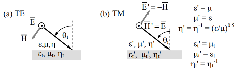
Figure 9.2.5(b) illustrates a TM plane wave incident upon a planar boundary where both the wave and the boundary conditions are dual to the TE wave illustrated in (a).

The behavior of TM waves at planar boundaries between non-conducting media is therefore characterized by duality transformations of Equations (9.2.62–65) for TE waves, supplemented by similar transformations of the expressions for the complex reflection and transmission coefficients \(\mathrm{\Gamma=\underline{E}_{r} / \underline{E}_{0}}), (9.2.28), and \( \mathrm{T}=\underline{\mathrm{E}}_{\mathrm{t}} / \underline{\mathrm{E}}_{\mathrm{o}}\), (9.2.29). After the transformations \(\overline{\mathrm{E}} \Rightarrow \overline{\mathrm{H}}\), \(\overline{\mathrm{H}} \Rightarrow-\overline{\mathrm{E}}\), and \(\varepsilon \Leftrightarrow \mu\), Equations (9.2.14–19) become:

\[\underline{\mathrm{\overline H}}_{\mathrm{i}}=\hat{y} \underline{\mathrm{H}}_{\mathrm{o}} \mathrm{e}^{\mathrm{jk}_{\mathrm{x}} \mathrm{x}-\mathrm{j} \mathrm{k}_{\mathrm{z}} \mathrm{z}} \ \left[\mathrm{Am}^{-1}\right]\]

\[\overline{\mathrm{\underline E}}_{\mathrm{i}}=\left(\underline{\mathrm{H}}_{\mathrm{o}} \eta\right)\left(\hat{x} \sin \theta_{\mathrm{i}}+\hat{z} \cos \theta_{\mathrm{i}}\right) \mathrm{e}^{\mathrm{j} \mathrm{k}_{\mathrm{x}} \mathrm{x}-\mathrm{j} \mathrm{k}_{\mathrm{z}} \mathrm{z}} \ \left[\mathrm{Vm}^{-1}\right]\]

\[\underline{\mathrm{\overline H}}_{\mathrm{r}}=\hat{y} \underline{\mathrm{H}}_{\mathrm{r}} \mathrm{e}^{-\mathrm{j} \mathrm{k}_{\mathrm{rx}} \mathrm{x}-\mathrm{j} \mathrm{k}_{\mathrm{z}} \mathrm{z}} \ \left[\mathrm{Am}^{-1}\right]\]

\[\overline{\mathrm{\underline E}}_{\mathrm{r}}=\left(\underline{\mathrm{H}}_{\mathrm{r}} \eta\right)\left(\hat{x} \sin \theta_{\mathrm{r}}-\hat{z} \cos \theta_{\mathrm{r}}\right) \mathrm{e}^{-\mathrm{j} \mathrm{k}_{\mathrm{rx}} \mathrm{x}-\mathrm{j} \mathrm{k}_{\mathrm{z}} \mathrm{z}} \ \left[\mathrm{Vm}^{-1}\right]\]

\[\overline{\mathrm{\underline H}}_{\mathrm{t}}=\hat{y} \underline{\mathrm{H}}_{\mathrm{t}} \mathrm{e}^{\mathrm{j} \mathrm{k}_{\mathrm{tx}} \mathrm{x}-\mathrm{j} \mathrm{k}_{\mathrm{z}} \mathrm{z}} \ \left[\mathrm{Am}^{-1}\right]\]

\[\overline{\mathrm{\underline E}}_{\mathrm{t}}=\left(\underline{\mathrm{H}}_{\mathrm{t}} \eta_{\mathrm{t}}\right)\left(\hat{x} \sin \theta_{\mathrm{t}}+\hat{z} \cos \theta_{\mathrm{t}}\right) \mathrm{e}^{\mathrm{jk}_{\mathrm{tx}} \mathrm{x}-\mathrm{j} \mathrm{k}_{\mathrm{z}} \mathrm{z}} \ \left[\mathrm{Vm}^{-1}\right]\]

The complex reflection and transmission coefficients for TM waves are transformed versions of (9.2.28) and (9.2.29), where we define a new angle-dependent \(\eta_{\mathrm{n}} \) by interchanging μ ↔ ε in \( \eta_{\mathrm{n}}^{\prime}\) in (9.2.28):

\[\underline{\mathrm{H}}_{\mathrm{r}} / \mathrm{\underline H}_{\mathrm{o}}=\left({\eta}_{\mathrm{n}}^{-1}-1\right) /\left({ }_{\eta}{ }_{\mathrm{n}}^{-1}+1\right)\]

\[\underline{\mathrm{H}}_{\mathrm{t}} / \underline{\mathrm{H}}_{\mathrm{o}}=2{\eta}_{\mathrm{n}}^{-1} /\left({ }_{\eta}{ }_{\mathrm{n}}^{-1}+1\right)\]

\[\eta_{\mathrm{n}}^{-1} \equiv \eta \cos \theta_{\mathrm{i}} /\left(\eta_{\mathrm{t}} \cos \theta_{\mathrm{t}}\right)\]

These equations, (9.2.66) to (9.2.74), completely describe the TM case, once phase matching provides θ_r and θ_t.

It is interesting to compare the power reflected for TE and TM waves as a function of the angle of incidence θ_i. Power in uniform plane waves is proportional to both \(|\overline{\mathrm{\underline E}}|^{2}\) and \( |\overline{\mathrm{\underline H}}|^{2}\). Figure 9.2.6 sketches how the fractional power reflected or surface reflectivity varies with angle of incidence θ_i for both TE and TM waves for various impedance mismatches, assuming \(\mu=\mu_{\mathrm{t}}\) and σ = 0 everywhere. If the wave is incident upon a medium with ε_t > ε, then \(|\underline{\Gamma}|^{2} \rightarrow 1\) as θ → 90^° , whereas \(|\underline \Gamma|^{2} \rightarrow 1\) at the critical angle θ_c if ε_t < ε, and remains unity for θ_c < θ < 90^o (this θ_c case is not illustrated).

Figure \(\PageIndex{6}\): Power reflected from planar dielectric interfaces for \(\mu=\mu_{\mathrm{t}}\).

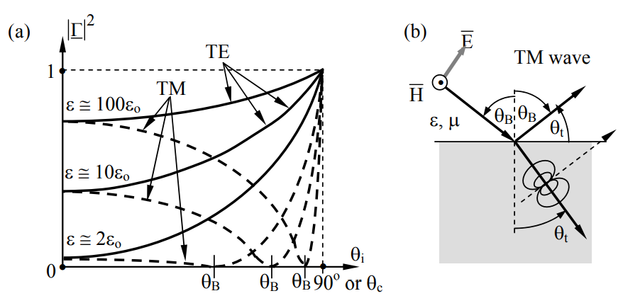
Figure 9.2.6 reveals an important phenomenon—there is perfect transmission at Brewster’s angle θ_B for one of the two polarizations. In this case Brewster’s angle occurs for the TM polarization because μ is the same everywhere and ε is not, and it would occur for TE polarization if μ varied across the boundary while ε did not. This phenomenon is widely used in glass Brewster-angle windows when even the slightest reflection must be avoided or when pure linear polarization is required (the reflected wave is pure).

We can compute θ_B by noting \(\underline{\mathrm{H}}_{\mathrm r} / \underline{\mathrm{H}}_{0}\) and, using (9.2.72), \( \eta_{\mathrm{n}}=1\). If μ = μ_t, then (9.2.74) yields \( \varepsilon_{\mathrm{t}}^{0.5} \cos \theta_{\mathrm{i}}=\varepsilon^{0.5} \cos \theta_{\mathrm{t}}\). Snell’s law for μ = μ_t yields \(\varepsilon^{0.5} \sin \theta_{i}=\varepsilon_{t}^{0.5} \sin \theta_{t}\). These two equations are satisfied if \(\sin \theta_{i}=\cos \theta_{t}\) and \(\cos \theta_{i}=\sin \theta_{t}\). Dividing this form of Snell’s law by \(\left[\cos \theta_{i}=\sin \theta_{t}\right]\) yields: \(\tan \theta_{\mathrm{i}}=\left(\varepsilon_{\mathrm{t}} / \varepsilon_{\mathrm{i}}\right)^{0.5}\), or:

\[\theta_{\mathrm{B}}=\tan ^{-1} \sqrt{\varepsilon_{\mathrm{t}} / \varepsilon_{\mathrm{i}}}\]

Moreover, dividing [sin θ_i = cos θ_t] by [cos θ_i = sin θ_t] yields tan θ_B = cos θ_t, which implies θ_B + θ_t = 90°. Using this equation it is easy to show that θ_B > 45^o for interfaces where θ_t < θ_i, and when θ_t > θ_i, it follows that θ_B < 45^o.

One way to physically interpret Brewster’s angle for TM waves is to note that at θ_B the polar axes of the electric dipoles induced in the second dielectric ε_t are pointed exactly at the angle of reflection mandated by phase matching, but dipoles radiate nothing along their polar axis; Figure 9.2.6(b) illustrates the geometry. That is, θ_B + θ_t = 90^o. For magnetic media magnetic dipoles are induced, and for TE waves their axes point in the direction of reflection at Brewster’s angle.

Yet another way to physically interpret Brewster’s angle is to note that perfect transmission can be achieved if the boundary conditions can be matched without invoking a reflected wave. This requires existence of a pair of incidence and transmission angles θ_i and θ_t such that the parallel components of both \(\overline{\mathrm{E}}\) and \(\overline{\mathrm{H}}\) for these two waves match across the boundary. Such a pair consistent with Snell’s law always exists for TM waves at planar dielectric boundaries, but not for TE waves. Thus there is perfect impedance matching at Brewster’s angle.

Example \(\PageIndex{E}\)

What is Brewster’s angle θ_B if μ₂ = 4μ₁, and ε₂ = ε₁, and for which polarization would the phenomenon be observed?

Solution

If the permeabilities differ, but not the permittivities, then Brewster’s angle is observed only for TE waves. At Brewster’s angle θ_B + θ_t = 90^°, and Snell’s law says \(\frac{\sin \theta_{\mathrm{t}}}{\sin \theta_{\mathrm{B}}}=\sqrt{\frac{\mu}{\mu_{\mathrm{t}}}}\). But \(\sin \theta_{\mathrm{t}}=\sin \left(90^{\circ}-\theta_{\mathrm{B}}\right)=\cos \theta_{\mathrm{B}}\), so Snell’s law becomes: \( \tan \theta_{\mathrm{B}}=\sqrt{\mu_{\mathrm{t}} / \mu}=2\) and \(\theta_{B} \cong 63^{\circ} \).