5.14: Mixed Dielectrics

This section addresses the question: If there are two or more dielectric media between the plates of a capacitor, with different permittivities, are the electric fields in the two media different, or are they the same? The answer depends on

1. Whether by “electric field” you mean \(E\) or \(D\);
2. The disposition of the media between the plates – i.e. whether the two dielectrics are in series or in parallel.

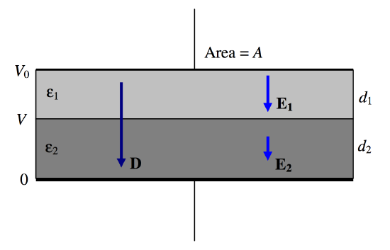
Let us first suppose that two media are in series (Figure \(V.\)16).

\(\text{FIGURE V.16}\)

Our capacitor has two dielectrics in series, the first one of thickness \(d_1\) and permittivity \(\epsilon_1\) and the second one of thickness \(d_2\) and permittivity \(\epsilon_2\). As always, the thicknesses of the dielectrics are supposed to be small so that the fields within them are uniform. This is effectively two capacitors in series, of capacitances \(\epsilon_1A/d_1 \text{ and }\epsilon_2A/d_2\). The total capacitance is therefore

\[C=\frac{\epsilon_1\epsilon_2A}{\epsilon_2d_1+\epsilon_1d_2}.\label{5.14.1}\]

Let us imagine that the potential difference across the plates is \(V_0\). Specifically, we’ll suppose the potential of the lower plate is zero and the potential of the upper plate is \(V_0\). The charge \(Q\) held by the capacitor (positive on one plate, negative on the other) is just given by \(Q = CV_0\), and hence the surface charge density \(\sigma\) is \(CV_0/A\). Gauss’s law is that the total \(D\)-flux arising from a charge is equal to the charge, so that in this geometry \(D = \sigma\), and this is not altered by the nature of the dielectric materials between the plates. Thus, in this capacitor, \(D = CV_0/A = Q/A\) in both media. Thus \(D\) is continuous across the boundary.

Then by application of \(D = \epsilon E\) to each of the media, we find that the \(E\)-fields in the two media are \(E_1\)=\(Q\)/\((\epsilon_1A\)) and \(E_2\)=\(Q\)/\((\epsilon_2A\)), the \(E\)-field (and hence the potential gradient) being larger in the medium with the smaller permittivity.

The potential V at the media boundary is given by \(V/d_2=E_2\). Combining this with our expression for \(E_2\), and \(Q = CV\)and Equation \ref{5.14.1}, we find for the boundary potential:

\[V=\frac{\epsilon_1d_2}{\epsilon_2d_1+\epsilon_1d_2}V_0.\label{5.14.2}\]

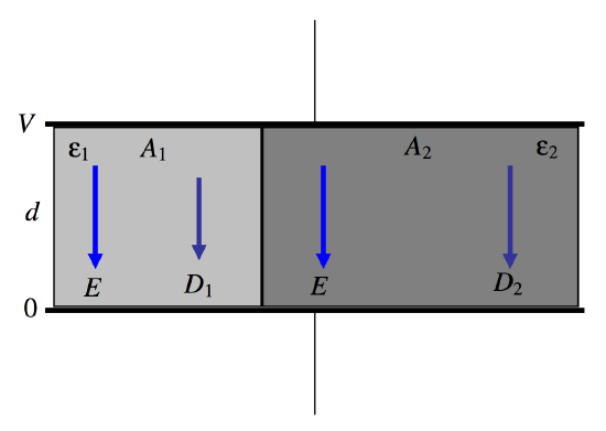
Let us now suppose that two media are in parallel (Figure \(V.\)17).

\(\text{FIGURE V.17}\)

This time, we have two dielectrics, each of thickness \(d\), but one has area \(A_1\) and permittivity \(\epsilon_1\) while the other has area \(A_2\) and permittivity \(\epsilon_2\). This is just two capacitors in parallel, and the total capacitance is

\[C=\frac{\epsilon_1A_1}{d}+\frac{\epsilon_2A_2}{d}\label{5.14.3}\]

The \(E\)-field is just the potential gradient, and this is independent of any medium between the plates, so that \(E = V/d\). in each of the two dielectrics. After that, we have simply that \(D_1=\epsilon_1E \text{ and }D_2=\epsilon_2E\). The charge density on the plates is given by Gauss’s law as \(\sigma = D\), so that, if \(\epsilon_1 < \epsilon_2\), the charge density on the left hand portion of each plate is less than on the right hand portion – although the potential is the same throughout each plate. (The surface of a metal is always an equipotential surface.) The two different charge densities on each plate is a result of the different polarizations of the two dielectrics – something that will be more readily understood a little later in this chapter when we deal with media polarization.

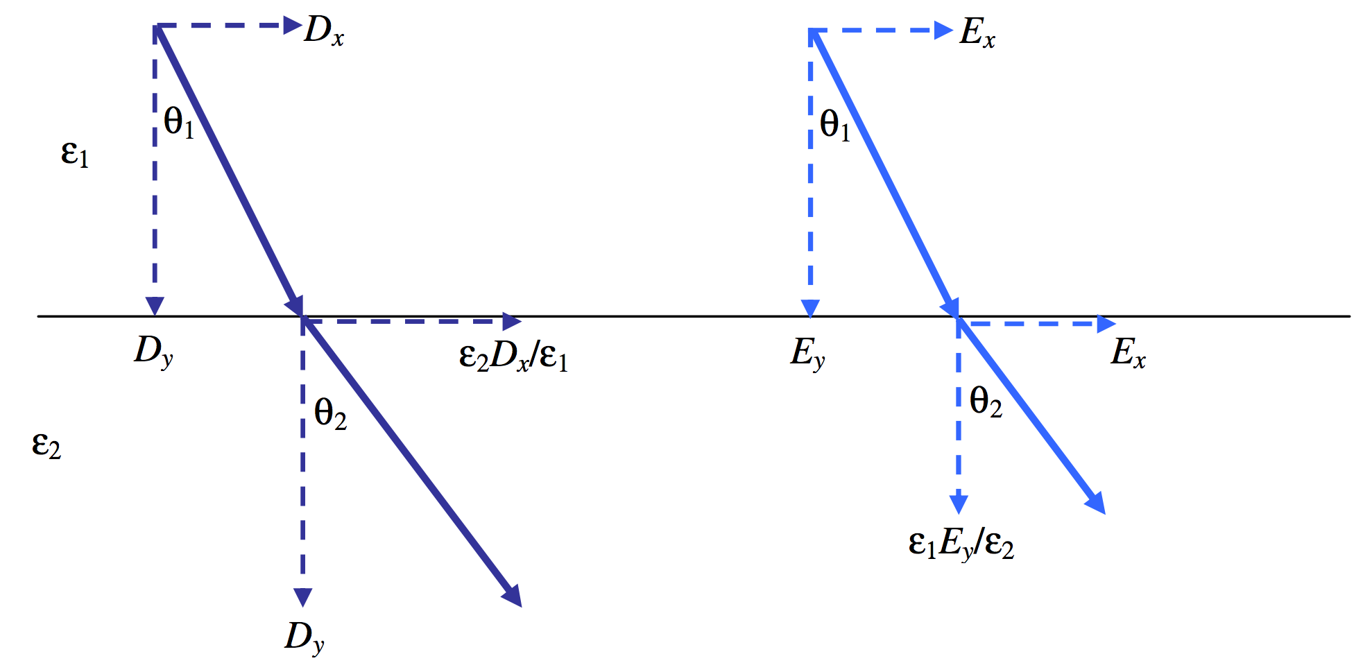
We have established that:

1. The component of \(\textbf{D}\) perpendicular to a boundary is continuous;
2. The component of \(\textbf{E}\) parallel to a boundary is continuous.

In Figure \(V.\)18 we are looking at the \(D\)-field and at the \(E\)-field as it crosses a boundary in which \(\epsilon_1 < \epsilon_2\). Note that \(D_y\) and \(E_x\)are the same on either side of the boundary. This results in:

\[\frac{\tan \theta_1}{\tan \theta_2}=\frac{\epsilon_1}{\epsilon_2}.\label{5.14.4}\]

\(\text{FIGURE V.18}\)