4.3: Boundary Problems

For an Ohmic conducting medium, we may combine Eqs. (6) and (8) to get the following differential equation

\[\ \nabla \cdot(\sigma \nabla \phi)=0.\tag{4.14}\]

For a uniform conductor \(\ (\sigma=\mathrm{const})\), Eq. (14) is reduced to the Laplace equation for the (macroscopic) electrostatic potential \(\ \phi\). As we already know from Chapters 2 and 3, its solution depends on the boundary conditions. These conditions, in turn, depend on the interface type.

(i) Conductor-conductor interface. Applying the continuity equation (6) to a Gauss-type pillbox at the interface of two different conductors (Fig. 5), we get

\[\ \left(j_{n}\right)_{1}=\left(j_{n}\right)_{2},\tag{4.15}\]

so that if the Ohm law (8) is valid inside each medium, then

\[\ \sigma_{1} \frac{\partial \phi_{1}}{\partial n}=\sigma_{2} \frac{\partial \phi_{2}}{\partial n}.\tag{4.16}\]

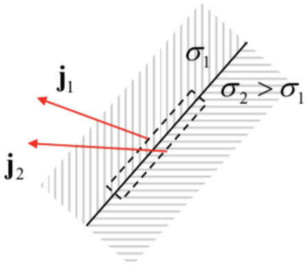Fig. 4.5. DC current’s “refraction” at the interface between two different conductors.

Also, since the electric field should be finite, its potential \(\ \phi\) has to be continuous across the interface – the condition that may also be written as

\[\ \frac{\partial \phi_{1}}{\partial \tau}=\frac{\partial \phi_{2}}{\partial \tau}.\tag{4.17}\]

Both these conditions (and hence the solutions of the boundary problems using them) are similar to those for the interface between two dielectrics – cf. Eqs. (3.46)-(3.47). Note that using the Ohm law, Eq. (17) may be rewritten as

\[\ \frac{1}{\sigma_{1}}\left(j_{\tau}\right)_{1}=\frac{1}{\sigma_{2}}\left(j_{\tau}\right)_{2}.\tag{4.18}\]

Comparing it with Eq. (15) we see that, generally, the current density’s magnitude changes at the interface: \(\ j_{1} \neq j_{2}\). It is also curious that if \(\ \sigma_{1} \neq \sigma_{2}\), the current line slope changes at the interface (Fig. 5), qualitatively similar to the refraction of light rays in optics – see Chapter 7.

(ii) Conductor-electrode interface. An electrode is defined as a body made of a “perfect conductor”, i.e. of a medium with \(\ \sigma \rightarrow \infty\). Then, at a fixed current density at the interface, the electric field in the electrode tends to zero, and hence it may be described by the equality

\[\ \phi=\phi_{j}=\mathrm{const},\tag{4.19}\]

where constants \(\ \phi_{j}\) may be different for different electrodes (numbered with index \(\ j\)). Note that with such boundary conditions, the Laplace boundary problem becomes exactly the same as in electrostatics – see Eq. (2.35) – and hence we can use all the methods (and some solutions :-) of Chapter 2 for finding the dc current distribution.

(iii) Conductor-insulator interface. For the description of a good insulator, we can use the equality \(\ \sigma=0\), so that Eq. (16) yields the following boundary condition,

\[\ \frac{\partial \phi}{\partial n}=0,\tag{4.20}\]

for the potential derivative inside the conductor. From the Ohm law (8) in the form \(\ \mathbf{j}=-\sigma \nabla \phi\), we see that this is just the very natural requirement for the dc current not to flow into an insulator. Now note that this condition makes the Laplace problem inside the conductor completely well-defined, and independent on the potential distribution in the adjacent insulator. On the contrary, due to the continuity of the electrostatic potential at the border, its distribution inside the surrounding insulator has to follow that inside the conductor.

Let us discuss this conceptual issue on the following (apparently, trivial) example: dc current in a uniform wire of length l and a cross-section of area \(\ A\). The reader certainly knows the answer:

\[\ I=\frac{V}{R}, \quad \text { where } R \equiv \frac{V}{I}=\frac{l}{\sigma A},\quad\quad\quad\quad\text{Uniform wire’s resistance}\tag{4.21}\]

where the constant \(\ R\) is called the resistance.¹⁴ However, let us derive this result formally from our theoretical framework. For the simple geometry shown in Fig. 6a, this is easy to do. Here the potential evidently has a linear 1D distribution

\[\ \phi=\text { const }-\frac{x}{l} V,\tag{4.22}\]

both in the conductor and the surrounding free space, with both boundary conditions (16) and (17) satisfied at the conductor-insulator interfaces, and the condition (20) satisfied at the conductor-electrode interfaces. As a result, the electric field is constant and has only one component \(\ E_{x}=V / l\), so that inside the conductor

\[\ j_{x}=\sigma E_{x}, \quad I=j_{x} A,\tag{4.23}\]

giving us the well-known Eq. (21).

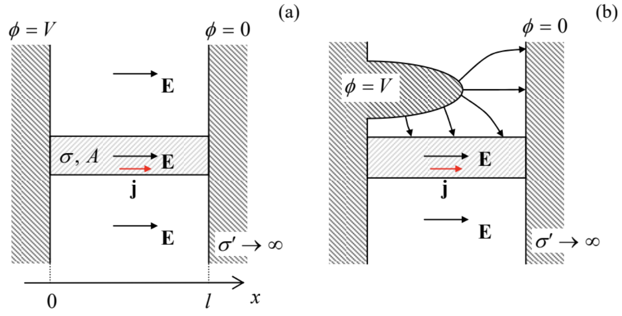Fig. 4.6. (a) An elementary problem and (b) a (slightly) less obvious problem of the field distribution at dc current flow (schematically).

However, what about the geometry shown in Fig. 6b? In this case, the field distribution in the free space around the conductor is dramatically different, but according to the boundary problem defined by Eqs. (14) and (20), inside the conductor, the solution is exactly the same as it was in the former case. Now, the Laplace equation in the surrounding insulator has to be solved with the boundary values of the electrostatic potential, “dictated” by the distribution of the current (and hence potential) in the conductor. Note that as the result, the electric field lines are generally not normal to the conductor’s surface, because the surface is not equipotential.

Let us solve a problem in that this conduction hierarchy may be followed analytically to the very end. Consider an empty spherical cavity carved in a conductor with an initially uniform current flow with a constant density \(\ \mathbf{j}_{0}=\mathbf{n}_{z} j_{0}\) (Fig. 7a). Following the hierarchy, we have to solve the boundary problem in the conducting part of the system, i.e. outside the sphere \(\ (r \geq R)\), first. Since the problem is evidently axially symmetric, we already know the general solution of the Laplace equation – see Eq. (2.172). Moreover, we know that in order to match the uniform field distribution at \(\ r \rightarrow \infty\), all coefficients \(\ a_{l}\) but one \(\ \left(a_{1}=-E_{0}=-j_{0} / \sigma\right)\) have to be zero, and that the boundary conditions at \(\ r=R\) will give zero solutions for all coefficients \(\ b_{l}\) but one \(\ \left(b_{1}\right)\), so that

\[\ \phi=-\frac{j_{0}}{\sigma} r \cos \theta+\frac{b_{1}}{r^{2}} \cos \theta, \quad \text { for } r \geq R.\tag{4.24}\]

In order to find the coefficient \(\ b_{1}\), we have to use the boundary condition (20) at \(\ r=R\):

\[\ \left.\frac{\partial \phi}{\partial r}\right|_{r=R}=\left(-\frac{j_{0}}{\sigma}-\frac{2 b_{1}}{R^{3}}\right) \cos \theta=0.\tag{4.25}\]

This gives \(\ b_{1}=-j_{0} R^{3} / 2 \sigma\), so that, finally,

\[\ \phi(r, \theta)=-\frac{j_{0}}{\sigma}\left(r+\frac{R^{3}}{2 r^{2}}\right) \cos \theta, \quad \text { for } r \geq R.\tag{4.26}\]

(Note that this potential distribution corresponds to the dipole moment \(\ \mathbf{p}=-\mathbf{E}_{0} R^{3} / 2\). It is straightforward to check that if the spherical cavity was cut in a dielectric, the potential distribution outside it would be similar, with \(\ \mathbf{p}=-\mathbf{E}_{0} R^{3}(\kappa-1) /(\kappa+2)\). In the limit \(\ \kappa \rightarrow \infty\), these two results coincide, despite the rather different type of the problem: in the dielectric case, there is no current at all.)

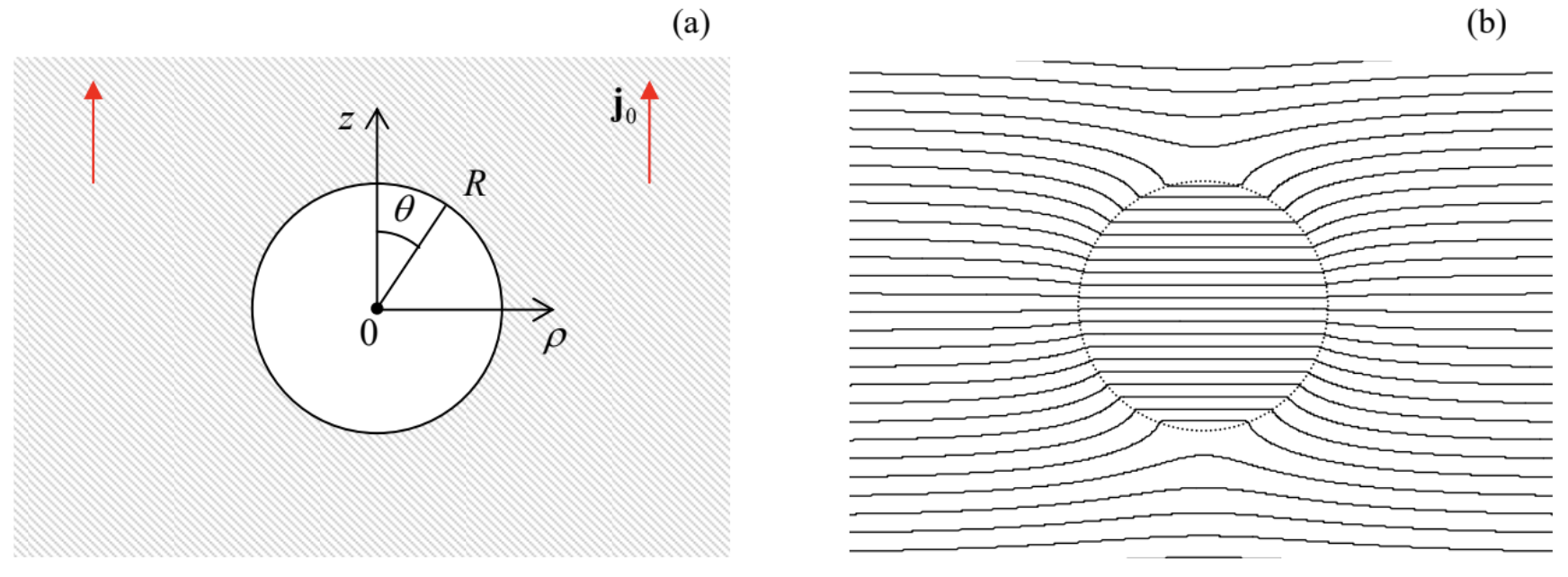Fig. 4.7. A spherical cavity carved in a uniform conductor: (a) the problem’s geometry, and (b) the equipotential surfaces as given by Eqs. (26) and (28).

Now, as the second step in the conductivity hierarchy, we may find the electrostatic potential distribution \(\ \phi(r, \theta)\) in the insulator, in this particular case inside the empty cavity \(\ (r \leq R)\). It should also satisfy the Laplace equation with the boundary values at \(\ r=R\), “dictated” by the distribution (26):

\[\ \phi(R, \theta)=-\frac{3}{2} \frac{j_{0}}{\sigma} R \cos \theta.\tag{4.27}\]

We could again solve this problem by the formal variable separation (keeping in the general solution (2.172) only the term proportional to \(\ a_{1}\), which does not diverge at \(\ r \rightarrow 0\)), but if we notice that the boundary condition (27) depends on just one Cartesian coordinate, \(\ z=R \cos \theta\), the solution may be just guessed:

\[\ \phi(r, \theta)=-\frac{3}{2} \frac{j_{0}}{\sigma} z=-\frac{3}{2} \frac{j_{0}}{\sigma} r \cos \theta, \quad \text { at } r \leq R.\tag{4.28}\]

Indeed, it evidently satisfies the Laplace equation and the boundary condition (27), and corresponds to a constant electric field parallel to the vector \(\ \mathbf{J}_{0}\), and equal to \(\ 3 j_{0} / 2 \sigma\) – see Fig. 7b. Again, the cavity surface it not equipotential, and the electric field lines at \(\ r \leq R\) are not normal to it at almost all points.

More generally, the conductivity hierarchy says that static electrical fields and charges outside conductors (e.g., electric wires) do not affect currents flowing in the wires, and it is physically very clear why. For example, if a charge in the free space is slowly moved close to a wire, it (in accordance with the linear superposition principle) only induces an additional surface charge (see Sec. 2.1) that screens the external charge’s field, without participating in the current flow inside the conductor.

Besides this conceptual issue, the two examples given above may be considered as applications of the first two methods discussed in Chapter 2 – the orthogonal coordinates (Fig. 6) and the variable separation (Fig. 7) – to dc current distribution problems. As the reader may recall, that chapter also discussed the method of charge images, and it may be also used for the solution of some dc conductivity problems. Indeed, let us consider the spherically-symmetric potential distribution of the electrostatic potential, similar to that given by the basic Eq. (1.35):

\[\ \phi=\frac{c}{r}.\tag{4.29}\]

As we know from Chapter 1, this is a particular solution of the 3D Laplace equation at all points but \(\ r=0\). In free space, this distribution would correspond to a point charge \(\ q=4 \pi \varepsilon_{0} c\); but what about a uniform Ohmic conductor? Calculating the corresponding electric field and current density,

\[\ \mathbf{E}=-\nabla \phi=\frac{c}{r^{3}} \mathbf{r}, \quad \mathbf{j}=\sigma \mathbf{E}=\sigma \frac{c}{r^{3}} \mathbf{r},\tag{4.30}\]

we see that the total current flowing from the origin through a sphere of an arbitrary radius \(\ r\) does not depend on the radius:

\[\ I=A j=4 \pi r^{2} j=4 \pi \sigma c.\tag{4.31}\]

Plugging the resulting coefficient \(\ c\) into Eq. (29), we get

\[\ \phi=\frac{I}{4 \pi \sigma r}.\tag{4.32}\]

Hence the Coulomb-type distribution of the electric potential in a conductor is possible (at least at some distance from the singular point \(\ r=0\)), and describes the dc current \(\ I\) flowing out of a small-size electrode – or into such an electrode if the coefficient \(\ c\) is negative. Such current injection may be readily implemented experimentally; think for example about an insulated wire with a small bare end, inserted into a poorly conducting soil – an important method in geophysical research.¹⁵

Now let the current injection point \(\ \mathbf{r^{\prime}}\) be close to a plane interface between the conductor and an insulator (Fig. 8). In this case, besides the Laplace equation, we should satisfy the boundary condition,

\[\ j_{n}=\sigma E_{n}=-\sigma \frac{\partial \phi}{\partial n}=0,\tag{4.33}\]

at the interface. It is clear that this can be done by replacing the insulator with an imaginary similar conductor with an additional current injection point, at the mirror image point \(\ \mathbf{r^{\prime\prime}}\). Note, however, that in contrast to the charge images, the sign of the imaginary current has to be similar, not opposite, to the initial one, so that the total electrostatic potential inside the conducting semi-space is

\[\ \phi(\mathbf{r})=\frac{I}{4 \pi \sigma}\left(\frac{1}{\left|\mathbf{r}-\mathbf{r}^{\prime}\right|}+\frac{1}{\left|\mathbf{r}-\mathbf{r}^{\prime \prime}\right|}\right).\tag{4.34}\]

(The image current’s sign would be opposite at the interface between a conductor with a moderate conductivity and a perfect conductor (“electrode”), whose potential should be virtually constant.)

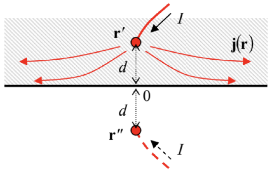Fig. 4.8. Applying the method of images for the current injection analysis.

This result may be readily used, for example, to calculate the current density at a plane surface of a uniform conductor, as a function of distance \(\ \rho\) from point 0, the surface’s point closest to the current injection site – see Fig. 8. At such surface, Eq. (34) yields

\[\ \phi=\frac{I}{2 \pi \sigma} \frac{1}{\left(\rho^{2}+d^{2}\right)^{1 / 2}},\tag{4.35}\]

so that the current density is:

\[\ j_{\rho}=\sigma E_{\rho}=-\sigma \frac{\partial \phi}{\partial \rho}=\frac{I}{2 \pi} \frac{\rho}{\left(\rho^{2}+d^{2}\right)^{3 / 2}}.\tag{4.36}\]

Deviations from Eqs. (35) and (36) may be used to find and characterize conductance inhomogeneities, say, those due to mineral deposits in the Earth’s crust.¹⁶

---

Reference

¹⁴ The first of Eqs. (21) is essentially the (historically, initial) integral form of the Ohm law, and is valid not only for a uniform wire, but also for Ohmic conductors of any geometry in that \(\ I\) and \(\ V\) may be clearly defined.

¹⁵ Such injection is even simpler in 2D situations – think about a wire soldered, in a small spot, to a thin conducting foil. (Note only that here the current density distribution law is different, \(\ j \propto 1 / r\) rather than \(\ 1 / r^{2}\).)

¹⁶ The current injection may be also produced, due to electrochemical reactions, by an ore mass itself, so that one need only measure (and correctly interpret :-) the resulting potential distribution – the so-called self-potential method – see, e.g., Sec. 6.1 in W. Telford et al., Applied Geophysics, 2^nd ed., Cambridge U. Press, 1990.