5.1: Magnetic Interaction of Currents

DC currents in conductors usually leave them electroneutral, \(\ \rho(\mathbf{r})=0\), with very good precision, because even a minute unbalance of positive and negative charge density results in extremely strong Coulomb forces that restore their balance by an additional shift of free charge carriers. This is why let us start the discussion of magnetism from the simplest case of two spatially-separated, dc-current-carrying, electroneutral conductors (Fig. 1).

Fig. 5.1. Magnetic interaction of two currents.

According to the Coulomb law, there is no electrostatic force between them. However, several experiments carried out in 1820¹ proved that there is a different, magnetic interaction between the currents. In the present-day notation, the results of all such experiments may be summarized with just one formula, in SI units expressed as:

\[\ \text{Magnetic force}\quad\quad\quad\quad\mathbf{F}=-\frac{\mu_{0}}{4 \pi} \int_{V} d^{3} r \int_{V^{\prime}} d^{3} r^{\prime}\left[\mathbf{j}(\mathbf{r}) \cdot \mathbf{j}^{\prime}\left(\mathbf{r}^{\prime}\right)\right] \frac{\mathbf{r}-\mathbf{r}^{\prime}}{\left|\mathbf{r}-\mathbf{r}^{\prime}\right|^{3}}\tag{5.1}\]

Here the coefficient \(\ \mu_{0} / 4 \pi\) (where \(\ \mu_{0}\) is called either the magnetic constant or the free space permeability) equals to almost exactly \(\ 10^{-7}\) SI units, with the product \(\ \varepsilon_{0} \mu_{0}\) equal to exactly \(\ 1 / c^{2}\).²

Note a close similarity of this expression to the Coulomb law (1.1), written for continuous charge distributions, with the account of the linear superposition principle (1.4):

\[\ \text{Electric force}\quad\quad\quad\quad\mathbf{F}=\frac{1}{4 \pi \varepsilon_{0}} \int_{V} d^{3} r \int_{V^{\prime}} d^{3} r^{\prime} \rho(\mathbf{r}) \rho^{\prime}\left(\mathbf{r}^{\prime}\right) \frac{\mathbf{r}-\mathbf{r}^{\prime}}{\left|\mathbf{r}-\mathbf{r}^{\prime}\right|^{3}}.\tag{5.2}\]

Besides the different coefficient and a different sign, the “only” difference of Eq. (1) from Eq. (2) is the scalar product of current densities, evidently necessary because of their vector character. We will see that this difference brings certain complications in applying the approaches discussed in the previous chapters, to magnetostatics.

Before going to their discussion, let us have one more glance at the coefficients in Eqs. (1) and (2). To compare them, let us consider two objects with uncompensated charge distributions \(\ \rho(\mathbf{r})\) and \(\ \rho^{\prime}(\mathbf{r})\), each moving parallel to each other as a whole, with certain velocities \(\ \mathbf{v}\) and \(\ \mathbf{v^{\prime}}\), as measured in the same inertial (“laboratory”) reference frame. In this case, \(\ \mathbf{j}(\mathbf{r})=\rho(\mathbf{r}) \mathbf{v}\), so that \(\ \mathbf{j}(\mathbf{r}) \cdot \mathbf{j}^{\prime}(\mathbf{r})=\rho(\mathbf{r}) \rho^{\prime}(\mathbf{r}) \nu \nu^{\prime}\), and the integrals in Eqs. (1) and (2) become functionally similar, differing only by the factor

\[\ \frac{F_{\text {magnetic }}}{F_{\text {electric }}}=-\frac{\mu_{0} \nu\nu^{\prime}}{4 \pi} / \frac{1}{4 \pi \varepsilon_{0}} \equiv-\frac{\nu \nu^{\prime}}{c^{2}}.\tag{5.3}\]

(The last expression is valid in any consistent system of units.) We immediately see that the magnetism is an essentially relativistic phenomenon, very weak in comparison with the electrostatic interaction at the human scale velocities, \(\ \nu<<c\), and may dominate only if the latter interaction vanishes – as it does in electroneutral systems.³ The discovery and initial studies⁴ of such a subtle, relativistic phenomenon as magnetism were much facilitated by the relative abundance of natural ferromagnets, materials with a spontaneous magnetic polarization, whose strong magnetic field is due to relativistic effects (such as spin) inside the constituent atoms – see Sec. 5 below.

Also, Eq. (3) points to an interesting paradox. Consider two electron beams moving parallel to each other, with the same velocity v with respect to a lab reference frame. Then, according to Eq. (3), the net force of their total (electric plus magnetic) interaction is proportional to \(\ \left(1-\nu^{2} / c^{2}\right)\), tending to zero in the limit \(\ \nu \rightarrow c\). However, in the reference frame moving together with the electrons, they are not moving at all, i.e. \(\ \nu=0\). Hence, from the point of view of such a moving observer, the electron beams should interact only electrostatically, with a repulsive force independent of the velocity \(\ \nu\). Historically, this had been one of several paradoxes that led to the development of special relativity; its resolution will be discussed in Chapter 9 devoted to this theory.

Returning to Eq. (1), in some simple cases the double integration in it may be carried out analytically. First of all, let us simplify this expression for the case of two thin, long conductors (“wires”) separated by a distance much larger than their thickness. In this case, we may integrate the products \(\ \mathbf{j} d^{3} r\) and \(\ \mathbf{j}^{\prime} d^{3} r^{\prime}\) over the wires’ cross-sections first, neglecting the corresponding change of the factor \(\ \left(\mathbf{r}-\mathbf{r}^{\prime}\right)\). Since the integrals of the current density over the cross-sections of the wires are just the currents \(\ I\) and \(\ I^{\prime}\) flowing in the wires, and cannot change along their lengths (say, \(\ l\) and \(\ l^{\prime}\), respectively), they may be taken out of the remaining integrals, reducing Eq. (1) to

\[\ \mathbf{F}=-\frac{\mu_{0} I I^{\prime}}{4 \pi} \oint_{l} \oint_{l^{\prime}}\left[d \mathbf{r} \cdot d \mathbf{r}^{\prime}\right] \frac{\mathbf{r}-\mathbf{r}^{\prime}}{\left|\mathbf{r}-\mathbf{r}^{\prime}\right|^{3}}.\tag{5.4}\]

As the simplest example, consider two straight, parallel wires (Fig. 2) separated by distance \(\ d\), both with length \(\ l >> d\).

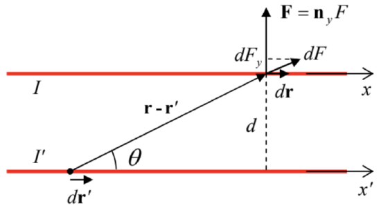Fig. 5.2. The magnetic force between two straight parallel currents.

In this case, due to symmetry, the vector of the magnetic interaction force has to:

(i) lie in the same plane as the currents, and

(ii) be normal to the wires – see Fig. 2.

Hence we may limit our calculations to just one component of the force – normal to the wires. Using the fact that with the coordinate choice shown in Fig. 2, the scalar product

\(\ d \mathbf{r} \cdot d \mathbf{r}^{\prime}\) is just \(\ d x d x\), we get

\[\ F=-\frac{\mu_{0} I I^{\prime}}{4 \pi} \int_{-\infty}^{+\infty} d x \int_{-\infty}^{+\infty} d x^{\prime} \frac{\sin \theta}{d^{2}+\left(x-x^{\prime}\right)^{2}}=-\frac{\mu_{0} I I^{\prime}}{4 \pi} \int_{-\infty}^{+\infty} d x \int_{-\infty}^{+\infty} d x^{\prime} \frac{d}{\left[d^{2}+\left(x-x^{\prime}\right)^{2}\right]^{3 / 2}}.\tag{5.5}\]

Now introducing, instead of \(\ x^{\prime}\), a new, dimensionless variable \(\ \xi \equiv\left(x-x^{\prime}\right) / d\), we may reduce the internal integral to a table one, which we have already encountered in this course:

\[\ F=-\frac{\mu_{0} I I^{\prime}}{4 \pi d} \int_{-\infty}^{+\infty} d x \int_{-\infty}^{+\infty} \frac{d \xi}{\left(1+\xi^{2}\right)^{3 / 2}}=-\frac{\mu_{0} I I^{\prime}}{2 \pi d} \int_{-\infty}^{+\infty} d x.\tag{5.6}\]

The integral over \(\ x\) formally diverges, but it gives a finite interaction force per unit length of the wires:

\[\ \frac{F}{l}=-\frac{\mu_{0} I I^{\prime}}{2 \pi d}.\tag{5.7}\]

Note that the force drops rather slowly (only as \(\ 1 / d\)) as the distance \(\ d\) between the wires is increased, and is attractive (rather than repulsive as in the Coulomb law) if the currents are of the same sign.

This is an important result,⁵ but again, the problems so simply solvable are few and far between, and it is intuitively clear that we would strongly benefit from the same approach as in electrostatics, i.e., from breaking Eq. (1) into a product of two factors via the introduction of a suitable field. Such decomposition may be done as follows:

\[\ \text{Lorentz force: current}\quad\quad\quad\quad\mathbf{F}=\int_{V} \mathbf{j}(\mathbf{r}) \times \mathbf{B}(\mathbf{r}) d^{3} r\tag{5.8}\]

where the vector \(\ \mathbf{B}\) is called the magnetic field.⁶ In the case when it is induced by the current \(\ \mathbf{j^{\prime}}\):

\[\ \mathbf{B}(\mathbf{r}) \equiv \frac{\mu_{0}}{4 \pi} \int_{V^{\prime}} \mathbf{j}^{\prime}\left(\mathbf{r}^{\prime}\right) \times \frac{\mathbf{r}-\mathbf{r}^{\prime}}{\left|\mathbf{r}-\mathbf{r}^{\prime}\right|^{3}} d^{3} r^{\prime}.\quad\quad\quad\quad\text{Biot-Savart
law}\tag{5.9}\]

The last relation is called the Biot-Savart law,⁷ while the force \(\ \mathbf{F}\) expressed by Eq. (8) is sometimes called the Lorentz force.⁸ However, more frequently the latter term is reserved for the full force,

\[\ \mathbf{F}=q(\mathbf{E}+\mathbf{v} \times \mathbf{B}),\quad\quad\quad\quad\text{Lorentz force: particle}\tag{5.10}\]

exerted by electric and magnetic fields field on a point charge \(\ q\), moving with velocity \(\ \mathbf{v}\).⁹

Now we have to prove that the new formulation, given by Eqs. (8)-(9), is equivalent to Eq. (1). At the first glance, this seems unlikely. Indeed, first of all, Eqs. (8) and (9) involve vector products, while Eq. (1) is based on a scalar product. More profoundly, in contrast to Eq. (1), Eqs. (8) and (9) do not satisfy the 3^rd Newton’s law applied to elementary current components \(\ \mathbf{j} d^{3} r\) and \(\ \text { j' } d^{3} r^{\prime}\), if these vectors are not parallel to each other. Indeed, consider the situation shown in Fig. 3.

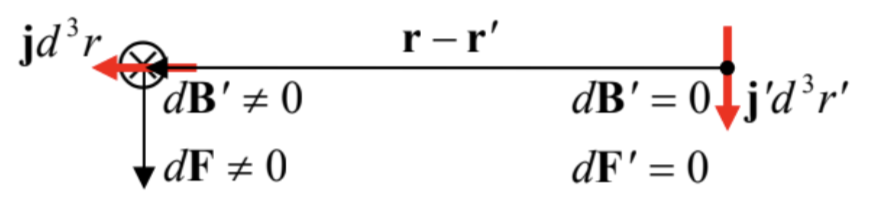Fig. 5.3. The apparent violation of the 3^rd Newton law in magnetism.

Here the vector \(\ \mathbf { j' }\) is perpendicular to the vector \(\ \left(\mathbf{r}-\mathbf{r}^{\prime}\right)\), and hence, according to Eq. (9), produces a non-zero contribution \(\ d \mathbf{B}^{\prime}\) to the magnetic field, directed (in Fig. 3) normally to the plane of the drawing, i.e. is perpendicular to the vector \(\ \mathbf{j}\). Hence, according to Eq. (8), this field provides a non-zero contribution to \(\ \mathbf{F}\). On the other hand, if we calculate the reciprocal force \(\ \mathbf{F}^{\prime}\) by swapping the prime indices in Eqs. (8) and (9), the latter equation immediately shows that \(\ d \mathbf{B}\left(\mathbf{r}^{\prime}\right) \propto \mathbf{j} \times\left(\mathbf{r}^{\prime}-\mathbf{r}\right)=0\), because the two operand vectors are parallel – see Fig. 3 again. Hence, the current component \(\ \mathbf{j}^{\prime} d^{3} \mathbf{r}^{\prime}\) does exert a force on its counterpart, while \(\ \mathbf{j} d^{3} \mathbf{r}\) does not.

Despite this apparent problem, let us still go ahead and plug Eq. (9) into Eq. (8):

\[\ \mathbf{F}=\frac{\mu_{0}}{4 \pi} \int_{V} d^{3} r \int_{V^{\prime}} d^{3} r^{\prime} \mathbf{j}(\mathbf{r}) \times\left(\mathbf{j}^{\prime}\left(\mathbf{r}^{\prime}\right) \times \frac{\mathbf{r}-\mathbf{r}^{\prime}}{\left|\mathbf{r}-\mathbf{r}^{\prime}\right|^{3}}\right).\tag{5.11}\]

This double vector product may be transformed into two scalar products, using the vector algebraic identity called the bac minus cab rule, \(\ \mathbf{a} \times(\mathbf{b} \times \mathbf{c})=\mathbf{b}(\mathbf{a} \cdot \mathbf{c})-\mathbf{c}(\mathbf{a} \cdot \mathbf{b})\).¹⁰ Applying this relation, with \(\ \mathbf{a}=\mathbf{j}\), \(\ \mathbf{b}=\mathbf{j}^{\prime}\), and \(\ \mathbf{c}=\mathbf{R} \equiv \mathbf{r}-\mathbf{r^{\prime}}\), to Eq. (11), we get

\[\ \mathbf{F}=\frac{\mu_{0}}{4 \pi} \int_{V^{\prime}} d^{3} r^{\prime} \mathbf{j}^{\prime}\left(\mathbf{r}^{\prime}\right)\left(\int_{V} d^{3} r \frac{\mathbf{j}(\mathbf{r}) \cdot \mathbf{R}}{R^{3}}\right)-\frac{\mu_{0}}{4 \pi} \int_{V} d^{3} r \int_{V^{\prime}} d^{3} r^{\prime} \mathbf{j}(\mathbf{r}) \cdot \mathbf{j}^{\prime}\left(\mathbf{r}^{\prime}\right) \frac{\mathbf{R}}{R^{3}}.\tag{5.12}\]

The second term on the right-hand side of this equality coincides with the right-hand side of Eq. (1), while the first term equals zero because its internal integral vanishes. Indeed, we may break the volumes \(\ V\) and \(\ V^{\prime}\) into narrow current tubes – the stretched elementary volumes whose walls are not crossed by
current lines (so that on their walls, \(\ j_{n}=0\). As a result, the elementary current in each tube, \(\ dI=jdA=j d^{2} r\), is the same along its length, and, just as in a thin wire, \(\ \mathbf{j} d^{2} r\) may be replaced with \(\ d I d \mathbf{r}\), with the vector \(\ d \mathbf{r}\) directed along \(\ \mathbf{j}\). Because of this, each tube’s contribution to the internal integral in the first term of Eq. (12) may be represented as

\[\ d I \oint_{l} d \mathbf{r} \cdot \frac{\mathbf{R}}{R^{3}}=-d I \oint_{l} d \mathbf{r} \cdot \nabla \frac{1}{R}=-d I \oint_{l} d r \frac{\partial}{\partial r} \frac{1}{R},\tag{5.13}\]

where the operator \(\ \nabla\) acts in the \(\ \mathbf{r}\)-space, and the integral is taken along the tube’s length \(\ l\). Due to the current continuity expressed by Eq. (4.6), each loop should follow a closed contour, and an integral of a full differential of some scalar function (in our case, 1/R) along such contour equals zero.

So we have recovered Eq. (1). Returning for a minute to the paradox illustrated with Fig. 3, we may conclude that the apparent violation of the 3^rd Newton law was the artifact of our interpretation of Eqs. (8) and (9) as the sums of independent elementary components. In reality, due to the dc current continuity, these components are not independent. For the whole currents, Eqs. (8)-(9) do obey the \(\ 3^{\mathrm{rd}}\) law – as follows from their already proved equivalence to Eq. (1).

Thus we have been able to break the magnetic interaction into two effects: the induction of the magnetic field \(\ \mathbf{B}\) by one current (in our notation, \(\ \mathbf{ j’ }\)), and the effect of this field on the other current (\(\ \mathbf{j}\)). Now comes an additional experimental fact: other elementary components \(\ \mathbf{j} d^{3} r^{\prime}\) of the current \(\ \mathbf{j}(\mathbf{r})\) also contribute to the magnetic field (9) acting on the component \(\ \mathbf{j} d^{3} r\).¹¹ This fact allows us to drop the prime sign after \(\ \mathbf{j}\) in Eq. (9), and rewrite Eqs. (8) and (9) as

\[\ \mathbf{B}(\mathbf{r})=\frac{\mu_{0}}{4 \pi} \int_{V^{\prime}} \mathbf{j}\left(\mathbf{r}^{\prime}\right) \times \frac{\mathbf{r}-\mathbf{r}^{\prime}}{\left|\mathbf{r}-\mathbf{r}^{\prime}\right|^{3}} d^{3} r^{\prime},\tag{5.14}\]

\[\ \mathbf{F}=\int_{V} \mathbf{j}(\mathbf{r}) \times \mathbf{B}(\mathbf{r}) d^{3} r.\tag{5.15}\]

Again, the field observation point r and the field source point \(\ \mathbf{r}^{\prime}\) have to be clearly distinguished. We immediately see that these expressions are close to, but still different from the corresponding relations of the electrostatics, namely Eq. (1.9) and the distributed-charge version of Eq. (1.6):

\[\ \mathbf{E}(\mathbf{r})=\frac{1}{4 \pi \varepsilon_{0}} \oint_{V^{\prime}} \rho\left(\mathbf{r}^{\prime}\right) \frac{\mathbf{r}-\mathbf{r}^{\prime}}{\left|\mathbf{r}-\mathbf{r}^{\prime}\right|^{3}} d^{3} r^{\prime},\tag{5.16}\]

\[\ \mathbf{F}=\oint_{V} \rho(\mathbf{r}) \mathbf{E}(\mathbf{r}) d^{3} r.\tag{5.17}\]

(Note that the sign difference has disappeared, at the cost of the replacement of scalar-by-vector multiplications in electrostatics with cross-products of vectors in magnetostatics.)

For the frequent case of a field of a thin wire of length \(\ l'\), Eq. (14) may be re-written as

\[\ \mathbf{B}(\mathbf{r})=\frac{\mu_{0} I}{4 \pi} \oint_{l^{\prime}} d \mathbf{r}^{\prime} \times \frac{\mathbf{r}-\mathbf{r}^{\prime}}{\left|\mathbf{r}-\mathbf{r}^{\prime}\right|^{3}}.\tag{5.18}\]

Let us see how does this formula work for the simplest case of a straight wire (Fig. 4a). The magnetic field contributions \(\ d \mathbf{B}\) due to all small fragments \(\ d \mathbf{r}^{\prime}\) of the wire’s length are directed along the same line (perpendicular to both the wire and the normal \(\ d\) dropped from the observation point to the wire’s line), and its magnitude is

\[\ d B=\frac{\mu_{0} I}{4 \pi} \frac{d x^{\prime}}{\left|\mathbf{r}-\mathbf{r}^{\prime}\right|^{2}} \sin \theta=\frac{\mu_{0} I}{4 \pi} \frac{d x^{\prime}}{\left(d^{2}+x^{2}\right)} \frac{d}{\left(d^{2}+x^{2}\right)^{1 / 2}}.\tag{5.19}\]

Summing up all such elementary contributions, we get

\[\ B=\frac{\mu_{0} I \rho}{4 \pi} \int_{-\infty}^{\infty} \frac{d x}{\left(x^{2}+d^{2}\right)^{3 / 2}}=\frac{\mu_{0} I}{2 \pi d}.\tag{5.20}\]

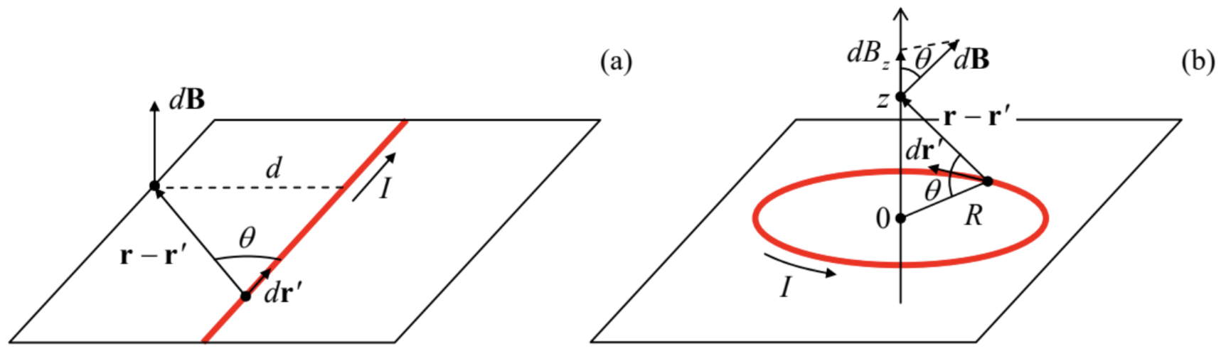Fig. 5.4. Calculating magnetic fields: (a) of a straight current, and (b) of a current loop.

This is a simple but important result. (Note that it is only valid for very long \(\ (l >> d)\), straight wires.) It is especially crucial to note the “vortex” character of the field: its lines go around the wire, forming rings with the centers on the current line. This is in sharp contrast to the electrostatic field lines, which can only begin and end on electric charges and never form closed loops (otherwise the Coulomb force \(\ q \mathbf{E}\) would not be conservative). In the magnetic case, the vortex structure of the field may be reconciled with the potential character of the magnetic forces, which is evident from Eq. (1), due to the vector products in Eqs. (14)-(15).

Now we may readily use Eq. (15), or rather its thin-wire version

\[\ \mathbf{F}=I \oint_{l} d \mathbf{r} \times \mathbf{B}(\mathbf{r}),\tag{5.21}\]

to apply Eq. (20) to the two-wire problem (Fig. 2). Since for the second wire vectors \(\ \mathrm{d} \mathbf{r}\) and \(\ \mathbf{B}\) are perpendicular to each other, we immediately arrive at our previous result (7), which was obtained directly from Eq. (1).

The next important example of the application of the Biot-Savart law (14) is the magnetic field at the axis of a circular current loop (Fig. 4b). Due to the problem’s symmetry, the net field \(\ \mathbf{B}\) has to be directed along the axis, but each of its elementary components \(\ \mathrm{d} \mathbf{B}\) is tilted by the angle \(\ \theta=\tan ^{-1}(z / R)\) to this axis, so that its axial component is

\[\ d B_{z}=d B \cos \theta=\frac{\mu_{0} I}{4 \pi} \frac{d r^{\prime}}{R^{2}+z^{2}} \frac{R}{\left(R^{2}+z^{2}\right)^{1 / 2}}.\tag{5.22}\]

Since the denominator of this expression remains the same for all wire components \(\ d r^{\prime}\), the integration over \(\ \mathbf{r}^{\prime}\) is easy \(\ (\int d r^{\prime}=2 \pi R)\), giving finally

\[\ B=\frac{\mu_{0} I}{2} \frac{R^{2}}{\left(R^{2}+z^{2}\right)^{3 / 2}}.\tag{5.23}\]

Note that the magnetic field in the loop’s center (i.e., for \(\ z=0\)),

\[\ B=\frac{\mu_{0} I}{2 R},\tag{5.24}\]

is \(\ \pi\) times higher than that due to a similar current in a straight wire, at distance \(\ d=R\) from it. This difference is readily understandable, since all elementary components of the loop are at the same distance \(\ R\) from the observation point, while in the case of a straight wire, all its points but one are separated from the observation point by distances larger than \(\ d\).

Another notable fact is that at large distances \(\ \left(z^{2} >> R^{2}\right)\), the field (23) is proportional to \(\ z^{-3}\):

\[\ B \approx \frac{\mu_{0} I}{2} \frac{R^{2}}{|z|^{3}} \equiv \frac{\mu_{0}}{4 \pi} \frac{2 m}{|z|^{3}}, \quad \text { with } m \equiv I A,\tag{5.25}\]

where \(\ A=\pi R^{2}\) is the loop area. Comparing this expression with Eq. (3.13), for the particular case \(\ \theta=0\), we see that such field is similar to that of an electric dipole (at least along its direction), with the replacement of the electric dipole moment magnitude \(\ p\) with the m so defined – besides the front factor. Indeed, such a plane current loop is the simplest example of a system whose field, at distances much larger than \(\ R\), is that of a magnetic dipole, with a dipole moment \(\ \mathbf{m}\) – the notions to be discussed in more detail in Sec. 4 below.

---

Reference

¹ Most notably, by Hans Christian Ørsted who discovered the effect of electric currents on magnetic needles, and André-Marie Ampère who has extended this work by finding the magnetic interaction between two currents.

² For details, see appendix CA: Selected Physical Constants. In the Gaussian units, the coefficient \(\ \mu_{0} / 4 \pi\) is replaced with \(\ 1 / c^{2}\).

³ An important case when the electroneutrality may not hold is the motion of electrons in vacuum. (However, in this case the electron speed is often comparable with the speed of light, so that the magnetic forces may be comparable in strength with electrostatic forces, and hence important.) In some semiconductor devices, local violations of electroneutrality also play an important role – see, e.g., SM Chapter 6.

⁴ The first detailed book on this subject, De Magnete by William Gilbert (a.k.a. Gilberd), was published as early as 1600.

⁵ In particular, until very recently (2018), Eq. (7) was used for the legal definition of the SI unit of current, one ampere (A), via the SI unit of force (the newton, N), with the coefficient \(\ \mu_{0}\) considered exactly fixed.

⁶ The SI unit of the magnetic field is called tesla (T) – after Nikola Tesla, a pioneer of electrical engineering. In the Gaussian units, the already discussed constant \(\ 1 / c^{2}\) in Eq. (1) is equally divided between Eqs. (8) and (9), so that in them both, the constant before the integral is \(\ 1 / c\). The resulting Gaussian unit of the field \(\ \mathbf{B}\) is called gauss (G); taking into account the difference of units of electric charge and length, and hence of the current density, 1 G equals exactly \(\ 10^{-4} \mathrm{~T}\). Note also that in some textbooks, especially old ones, \(\ \mathbf{B}\) is called either the magnetic induction or the magnetic flux density, while the term “magnetic field” is reserved for the field \(\ \mathbf{H}\) that will be introduced in Sec. 5 below.

⁷ Named after Jean-Baptiste Biot and Félix Savart who made several key contributions to the theory of magnetic interactions – in the same notorious 1820.

⁸ Named after Hendrik Antoon Lorentz, famous mostly for his numerous contributions to the development of special relativity – see Chapter 9 below. To be fair, the magnetic part of the Lorentz force was implicitly described in a much earlier (1865) paper by J. C. Maxwell, and then spelled out by Oliver Heaviside (another genius of electrical engineering – and mathematics!) in 1889, i.e. also before the 1895 work by H. Lorentz.

⁹ From the magnetic part of Eq. (10), Eq. (8) may be derived by the elementary summation of all forces acting on \(\ n >> 1\) particles in a unit volume, with \(\ \mathbf{j}=q n \mathbf{v}\) – see the footnote on Eq. (4.13a). On the other hand, the reciprocal derivation of Eq. (10) from Eq. (8) with \(\ \mathbf{j}=q \mathbf{v} \delta\left(\mathbf{r}-\mathbf{r}_{0}\right)\), where \(\ \mathbf{r}_{0}\) is the current particle’s position (so that \(\ d \mathbf{r}_{0} / d t=\mathbf{v}\)), requires care and will be performed in Chapter 9.

¹⁰ See, e.g., MA Eq. (7.5).

¹¹ Just as in electrostatics, one needs to exercise due caution transforming these expressions for the limit of discrete classical particles, and extended wavefunctions in quantum mechanics, to avoid the (non-existing) magnetic interaction of a charged particle with itself.