
5.6: Systems with Magnetics


- Last updated
- Mar 5, 2022
- Save as PDF

( \newcommand{\kernel}{\mathrm{null}\,}\)
Similarly to the electrostatics of linear dielectrics, the magnetostatics of linear magnetics is very simple in the particular case when the stand-alone currents are embedded into a medium with a constant permeability μ. Indeed, let us assume that we know the solution B0(r) of the magnetic pair of the genuine (“microscopic”) Maxwell equations (36) in free space, i.e. when the genuine current density j coincides with that of stand-alone currents. Then the macroscopic Maxwell equations (109) and the linear constitutive equation (110) are satisfied with the pair of functions
H(r)=B0(r)μ0,B(r)=μH(r)=μμ0B0(r).
Hence the only effect of the complete filling of a fixed-current system with a uniform, linear magnetic is the change of the magnetic field B at all points by the same constant factor μ/μ0≡1+χm, which may be either larger or smaller than 1. (As a reminder, a similar filling of a system of fixed stand-alone charges with a uniform, linear dielectric always leads to a reduction of the electric field E by a factor of ε/ε0≡1+χe – the difference whose physics was already discussed at the end of Sec. 4.)
However, this simple result is generally invalid in the case of nonuniform (or piecewise-uniform) magnetic samples. To analyze this case, let us first integrate the macroscopic Maxwell equation (107) along a closed contour C limiting a smooth surface S. Now using the Stokes theorem, we get the macroscopic version of the Ampère law (37):
Macroscopic Ampère law∮CH⋅dr=I.
Let us apply this relation to a sharp boundary between two regions with different magnetics, with no stand-alone currents on the interface, similarly to how this was done for the field E in Sec. 3.4 – see Fig. 3.5. The result is similar as well:
Hτ= const .
On the other hand, the integration of the Maxwell equation (29) over a Gaussian pillbox enclosing a border fragment (again just as shown in Fig. 3.5 for the field D) yields the result similar to Eq. (3.35):
Bn= const .
For linear magnetics, with B=μH, the latter boundary condition is reduced to
μHn= const .
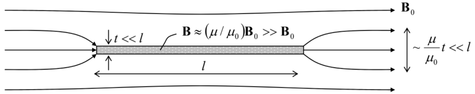
Let us use these boundary conditions, first of all, to see what happens with a long cylindrical sample of a uniform magnetic material, placed parallel to a uniform external magnetic field B0 – see Fig.15. Such a sample cannot noticeably disturb the field in the free space outside it, at most of its length: Bext=B0,Hext=μ0Bext=μ0B0. Now applying Eq. (117) to the dominating, side surfaces of the sample, we get Hint =H0.57 For a linear magnetic, these relations yield Bint =μHint =(μ/μ0)B0.58 For the high- μ, soft ferromagnetic materials, this means that Bint>>B0. This effect may be vividly represented as the concentration of the magnetic field lines in high- μ samples – see Fig. 15 again. (The concentration affects the external field distribution only at distances of the order of (μ/μ0)t<<l near the sample’s ends.) Such concentration is widely used in such practically important devices as transformers, in which two multi-turn coils are wound on a ring-shaped (e.g., toroidal, see Fig. 6b) core made of a soft ferromagnetic material (such as the transformer steel, see Table 1) with μ>>μ0. This minimizes the number of “stray” field lines, and makes the magnetic flux Φ piercing each wire turn (of either coil) virtually the same – the equality important for the secondary voltage induction – see the next chapter.
Samples of other geometries may create strong perturbations of the external field, extended to distances of the order of the sample’s dimensions. To analyze such problems, we may benefit from a simple, partial differential equation for a scalar function, e.g., the Laplace equation, because in Chapter 2 we have learned how to solve it for many simple geometries. In magnetostatics, the introduction of a scalar potential is generally impossible due to the vortex-like magnetic field lines. However, if there are no stand-alone currents within the region we are interested in, then the macroscopic Maxwell equation (107) for the field H is reduced to ∇×H=0, similar to Eq. (1.28) for the electric field, showing that we may introduce the scalar potential of the magnetic field, ϕm, using the relation similar to Eq. (1.33):
H=−∇ϕm.
Combining it with the homogenous Maxwell equation (29) for the magnetic field, ∇⋅B=0, and Eq.(110) for a linear magnetic, we arrive at a single differential equation, ∇⋅(μ∇ϕm)=0. For a uniform medium (μ(r)=const), it is reduced to our beloved Laplace equation:
∇2ϕm=0.
Moreover, Eqs. (117) and (119) give us very familiar boundary conditions: the first of them
∂ϕm∂τ=const,
being equivalent to
ϕm= const ,
while the second one giving
μ∂ϕm∂n=const.
Indeed, these boundary conditions are absolutely similar for (3.37) and (3.56) of electrostatics, with the replacement ε→μ.59
Let us analyze the geometric effects on magnetization, first using the (too?) familiar structure: a sphere, made of a linear magnetic material, placed into a uniform external field H0≡B0/μ0. Since the differential equation and the boundary conditions are similar to those of the corresponding electrostatics problem (see Fig. 3.11 and its discussion), we can use the above analogy to reuse the solution we already have – see Eqs. (3.63). Just as in the electric case, the field outside the sphere, with
(ϕm)r>R=H0(−r+μ−μ0μ+2μ0R3r2)cosθ,
is a sum of the uniform external field H0, with the potential −H0rcosθ≡−H0z, and the dipole field (99) with the following induced magnetic dipole moment of the sphere:60
m=4πμ−μ0μ+2μ0R3H0.
On the contrary, the internal field is perfectly uniform, and directed along the external one:
(ϕm)r<R=−H03μ0μ+2μ0rcosθ, so that HintH0=3μ0μ+2μ0,BintB0=μHintμ0H0=3μμ+2μ0.
Note that the field Hint inside the sphere is not equal to the applied external field H0. This example shows that the interpretation of H as the “would-be” magnetic field generated by external stand-alone currents j should not be exaggerated into saying that its distribution is independent of the magnetic bodies in the system. In the limit μ>>μ0, Eqs. (126) yield Hint /H0<<1,Bint /H0=3μ0, the factor 3 being specific for the particular geometry of the sphere. If a sample is strongly stretched along the applied field, with its length l much larger than the scale t of its cross-section, this geometric effect is gradually decreased, and Bint tends to its value μH0>>B0, as was discussed above – see Fig. 15.
Now let us calculate the field distribution in a similar, but slightly more complex (and practically important) system: a round cylindrical shell, made of a linear magnetic, placed into a uniform external field H0 normal to its axis – see Fig. 16.
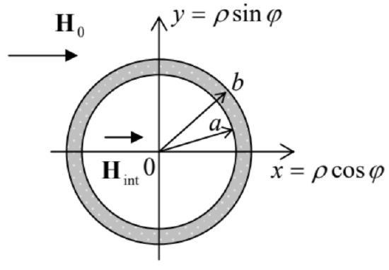 Fig. 5.16. Cylindrical magnetic shield.
Since there are no stand-alone currents in the region of our interest, we can again represent the field H(r) by the gradient of the magnetic potential ϕm – see Eq. (120). Inside each of three constant- μ regions, i.e. at ρ<b,a<ρ<b, and b<ρ (where ρ is the distance from the cylinder's axis), the potential obeys the Laplace equation (121). In the convenient, polar coordinates (see Fig. 16), we may, guided by the general solution (2.112) of the Laplace equation and our experience in its application to axially-symmetric geometries, look for ϕm in the following form:
ϕm={(−H0ρ+b′1/ρ)cosφ, for b≤ρ,(a1ρ+b1/ρ)cosφ, for a≤ρ≤b,−Hint ρcosφ, for ρ≤a.
Plugging this solution into the boundary conditions (122)-(123) at both interfaces ( ρ=b and ρ=a), we get the following system of four equations:
−H0b+b′1/b=a1b+b1/b,(a1a+b1/a)=−Hinta,μ0(−H0−b′1/b2)H0=μ(a1−b1/b2),μ(a1−b1/a2)=−μ0Hint,
for four unknown coefficients a1,b1,b′1, and Hint . Solving the system, we get, in particular:
HintH0=αc−1αc−(a/b)2, with αc≡(μ+μ0μ−μ0)2.
According to these formulas, at μ>μ0, the field in the free space inside the cylinder is lower than the external field. This fact allows using such structures, made of high- μ materials such as permalloy (see Table 1), for passive shielding61 from unintentional magnetic fields (e.g., the Earth's field) – the task very important for the design of many physical experiments. As Eq. (129) shows, the larger is μ, the closer is αc to 1, and the smaller is the ratio Hint/H0, i.e. the better is the shielding (for the same a/b ratio). On the other hand, for a given magnetic material, i.e. for a fixed parameter αc, the shielding is improved by making the ratio a/b<1 smaller, i.e. the shield thicker. On the other hand, as Fig. 16 shows, smaller a leaves less space for the shielded samples, calling for a compromise.
Now let us discuss a curious (and practically important) approach to systems with relatively thin, closed magnetic cores made of several sections of (possibly, different) high- μ magnetics, with the cross-section areas Ak much smaller than the squared lengths lk of the sections – see Fig. 17.
 Fig. 5.17. Deriving the “magnetic Ohm law” (131).
If all μk>>μ0, virtually all field lines are confined to the interior of the core. Then, applying the macroscopic Ampère law (116) to a contour C that follows a magnetic field line inside the core (see, for example, the dashed line in Fig. 17), we get the following approximate expression (exactly valid only in the limit μk/μ0,l2k/Ak→∞):
∮CHldl≈∑klkHk≡∑klkBkμk=NI.
However, since the magnetic field lines stay in the core, the magnetic flux Φk≈BkAk should be the same (≡Φ) for each section, so that Bk=Φ/Ak. Plugging this condition into Eq. (130), we get
Magnetic Ohm law and reluctanceΦ=NI∑kRk, where Rk≡lkμkAk.
Note a close analogy of the first of these equations with the usual Ohm law for several resistors connected in series, with the magnetic flux playing the role of electric current, while the product NI, the role of the voltage applied to the chain of resistors. This analogy is fortified by the fact that the second of Eqs. (131) is similar to the expression for the resistance R=l/σA of a long, uniform conductor, with the magnetic permeability μ playing the role of the electric conductivity σ. (To sound similar, but still different from the resistance R, the parameter R is called reluctance.) This is why Eq. (131) is called the magnetic Ohm law; it is very useful for approximate analyses of systems like ac transformers, magnetic energy storage systems, etc.
Now let me proceed to a brief discussion of systems with permanent magnets. First of all, using the definition (108) of the field H, we may rewrite the Maxwell equation (29) for the field B as
∇⋅B≡μ0∇⋅(H+M)=0, i.e. as ∇⋅H=−∇⋅M,
While this relation is general, it is especially convenient in permanent magnets, where the magnetization vector M may be considered field-independent. In this case, Eq. (132) for H is an exact analog of Eq. (1.27) for E, with the fixed term −∇⋅M playing the role of the fixed charge density (more exactly, of ρ/ε0). For the scalar potential ϕm, defined by Eq. (120), this gives the Poisson equation
∇2ϕm=∇⋅M,
similar to those solved, for quite a few geometries, in the previous chapters.
In the particular case when M is not only field-independent, but also uniform inside a permanent magnet’s volume, then the right-hand sides of Eqs. (132) and (133) vanish both inside the volume and in the surrounding free space, and give a non-zero effective charge only on the magnet’s surface. Integrating Eq. (132) along a short path normal to the surface and crossing it, we get the following boundary conditions:
ΔHn≡(Hn)in free space −(Hn)in magnet =Mn≡Mcosθ,
where θ is the angle between the magnetization vector and the outer normal to the magnet’s surface. This relation is an exact analog of Eq. (1.24) for the normal component of the field E, with the effective surface charge density (or rather σ/ε0) equal to Mcosθ.
This analogy between the magnetic field induced by a fixed, constant magnetization and the electric field induced by surface electric charges enables one to reuse quite a few problems considered in Chapters 1-3. Leaving a few such problems for the reader's exercise (see Sec. 7), let me demonstrate the power of this analogy on just two examples specific to magnetic systems. First, let us calculate the force necessary to detach the flat ends of two long, uniform rod magnets, of length l and cross-section area A<<l2, with the saturated remanent magnetization M0 directed along their length – see Fig. 18.
 Fig. 5.18. Detaching two magnets.
Let us assume we have succeeded to detach the magnets by an infinitesimal distance τ<<A1/2, l. Then, according to Eqs. (133)-(134), the distribution of the magnetic field near this small gap should be similar to that of the electric field in a system of two equal by opposite surface charges with the surface density σ proportional to M0. From Chapters 1 and 2, we know the properties of such a system very well: within the gap, the electric field is virtually constant, uniform, proportional to σ, and independent of τ. For its magnitude, Eq. (134) gives simply H=M0, and hence B=μ0M0. (Just outside of the gap, the field is very low, because due to the condition A<<l2, the effect of the similar effective charges at the "outer" ends of the rods on the field near the gap t is negligible.)
Now we could calculate Fmin as the force exerted by this field on the effective surface "charges". However, it is even easier to find it from the following energy argument. Since the magnetic field energy localized inside the magnets and near their outer ends cannot depend on t, this small detachment may only alter the energy inside the gap. For this part of the energy, Eq. (57) yields:
ΔU=B22μ0V=(μ0M0)22μ0Aτ.
The gradient of this potential energy is equal to the attraction force F=−∇(ΔU), trying to reduce ΔU by decreasing the gap, with the magnitude
|F|=∂(ΔU)∂τ=μ0M20A2.
The magnet detachment requires an equal and opposite external force.
Now let us consider the situation when similar long permanent magnets (such as the magnetic needles used in magnetic compasses) are separated, in otherwise free space, by a larger distance d>>A1/2 – see Fig. 19. For each needle (Fig. 19a), of a length l>>A1/2, the right-hand side of Eq. (133) is substantially different from zero only in two relatively small areas at the needle’s ends. Integrating the equation over each end, we see that at distances r>>A1/2 from each end, we may reduce Eq. (132) to
∇⋅H=qmδ(r−r+)−qmδ(r−r−),
where r± are ends’ positions, and qm≡M0A, with A being the needle’s cross-section area. This equation is completely similar to Eq. (3.32) for the displacement D, for the particular case of two equal and opposite point charges, i.e. with ρ=qδ(r−r+)−qδ(r−r+), with the only replacement q→qm. Since we know the resulting electric field all too well (see, e.g., Eq. (1.7) for E≡D/ε0), we may immediately write the similar expression for the field H:
H(r)=14πqm(r−r+|r−r+|3−r−r−|r−r−|3).
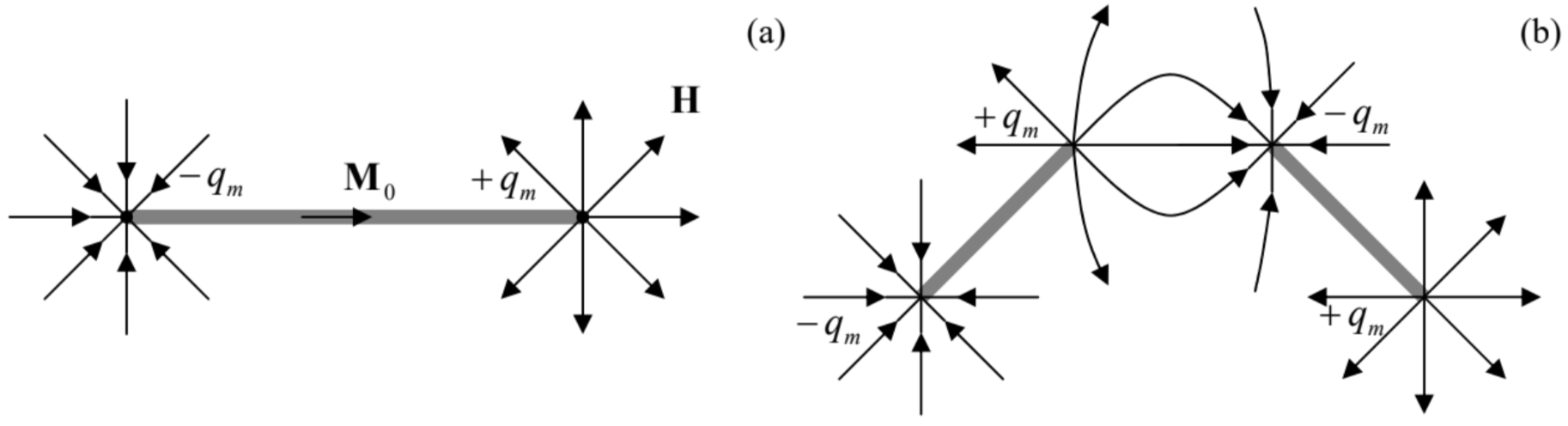 Fig. 5.19. (a) “Magnetic charges” at the ends of a thin permanent-magnet needle and (b) the result of its breaking into two parts (schematically).
The resulting magnetic field B(r)=μ0H(r) exerts on another “magnetic charge” q′m, located at
point r′, force F=q′mB(r′).62 Hence if two ends of different needles are separated by an intermediate distance R ( A1/2<<R<<l, see Fig. 19b), we may neglect one term in Eq. (138), and get the following “magnetic Coulomb law” for the interaction of the nearest ends:
F=±μ04πqmq′mRR3.
The “only” (but conceptually, crucial!) difference of this interaction from that of the electric point charges is that the two “magnetic charges” (quasi-monopoles) of a magnetic needle cannot be fully separated. For example, if we break the needle in the middle in at attempt to bring its two ends further apart, two new “point charges” appear – see Fig. 19b.
There are several solid-state systems where more flexible structures, similar in their magnetostatics to the needles, may be implemented. First of all, certain (“type-II”) superconductors may carry so-called Abrikosov vortices – flexible tubes with field-suppressed superconductivity inside, each carrying one quantum Φ0=πℏ/e≈2×10−15 Wb of the magnetic flux. Ending on superconductor’s surfaces, these tubes let their magnetic field lines spread into the surrounding free space, essentially forming magnetic monopole analogs – of course, with equal and opposite “magnetic charges” qm on each end of the tube – just as Fig. 19a shows. Such flux tubes are not only flexible but also stretchable, resulting in several peculiar effects – see Sec. 6.4 for more detail. Another recently found example of such paired quasi-monopoles is spin chains in the so-called spin ices – crystals with paramagnetic ions arranged into a specific (pyrochlore) lattice – such as dysprosium titanate Dy2Ti2O7.63 Let me emphasize again that any reference to magnetic monopoles in such systems should not be taken literally.
In order to complete this section (and this chapter), let me briefly discuss the magnetic field energy U, for the simplest case of systems with linear magnetics. In this case, we still may use Eq. (55), but if we want to operate with the macroscopic fields, and hence the stand-alone currents, we should repeat the manipulations that have led us to Eq. (57), using j not from Eq. (35), but from Eq. (107). As a result, instead of Eq. (57) we get
U=∫Vu(r)d3r, with u=B⋅H2=B22μ=μH22,Field energy in a linear magnetic
This result is evidently similar to Eq. (3.73) of electrostatics.
As a simple but important example of its application, let us again consider a long solenoid (Fig. 6a), but now filled with a linear magnetic material with permeability μ. Using the macroscopic Ampère law (116), just as we used Eq. (37) for the derivation of Eq. (40), we get
H=In, and hence B=μIn,
where n≡N/l, just as in Eq. (40), is the winding density, i.e. the number of wire turns per unit length. (At μ=μ0, we immediately return to that old result.) Now we may plug Eq. (141) into Eq. (140) to calculate the magnetic energy stored in the solenoid:
U=uV=μH22lA=μ(nI)2lA2,
and then use Eq. (72) to calculate its self-inductance:64
L=UI2/2=μn2lA
We see that L∝μV, so that filling a solenoid with a high- μ material may allow making it more compact while preserving the same value of inductance. In addition, as the discussion of Fig. 15 has shown, such filling reduces the fringe fields near the solenoid's ends, which may be detrimental for some applications, especially in physical experiments striving for high measurement precision.
However, we still need to explore the issue of magnetic energy beyond Eq. (140), not only to get a general expression for it in materials with an arbitrary dependence B(H), but also to finally prove Eq. (54) and explore its relation with Eq. (53). I will do this at the beginning of the next chapter.
Reference
57 The independence of H on magnetic properties of the sample in this geometry explains why this field’s magnitude is commonly used as the argument in the plots like Fig. 14: such measurements are typically carried out by placing an elongated sample of the material under study into a long solenoid with a controllable current I, so that according to Eq. (116), H0=nI, regardless of the sample.
58 The reader is highly encouraged to carry out a similar analysis of the fields inside narrow gaps cut in a linear magnetic, similar to that carried in Sec. 3.3 out for linear dielectrics – see Fig. 3.6 and its discussion.
59 This similarity may seem strange because earlier we have seen that the parameter μ is physically more similar to 1/ε. The reason for this paradox is that in magnetostatics, the magnetic potential ϕm is traditionally used to describe the “would-be field” H, while in electrostatics, the potential ϕ describes the actual electric field E. (This tradition persists from the days when H was perceived as a genuine magnetic field.)
60 To derive Eq. (125), we may either calculate the gradient of the ϕm given by Eq. (124), or use the similarity of Eqs. (3.13) and (99), to derive from Eq. (3.17) a similar expression for the magnetic dipole’s potential
ϕm=14πmcosθr2.
Now comparing this formula with the second term of Eq. (124), we immediately get Eq. (125).
61 Another approach to the undesirable magnetic fields' reduction is the "active shielding" – the external field’s compensation with the counter-field induced by controlled currents in specially designed wire coils.
62 The simplest way to verify this (perhaps, obvious) expression is to check that for a system of two “charges” ±q′m, separated by vector a, placed into a uniform external magnetic field Bext , it yields the potential energy (100) with the correct magnetic dipole moment m=qma – cf. Eq. (3.9) for an electric dipole.
63 See, e.g., L. Jaubert and P. Holdworth, J. Phys. – Cond. Matt. 23, 164222 (2011), and references therein.
64 Admittedly, we could get the same result simpler, just by arguing that since the magnetic material fills the whole volume of a substantial magnetic field in this system, the filling simply increases the vector B at all points, and hence its flux Φ, and hence L≡Φ/I by the factor μ/μ0 in comparison with the free-space value (75).