5.2: Vector Potential and the Ampère Law

The reader could see that the calculations of the magnetic field using Eq. (14) or (18) are still somewhat cumbersome even for the very simple systems we have examined. As we saw in Chapter 1, similar calculations in electrostatics, at least for several important systems of high symmetry, could be substantially simplified using the Gauss law (1.16). A similar relation exists in magnetostatics as well, but has a different form, due to the vortex character of the magnetic field.

To derive it, let us notice that in an analogy with the scalar case, the vector product under the integral (14) may be transformed as

\[\ \frac{j\left(\mathbf{r}^{\prime}\right) \times\left(\mathbf{r}-\mathbf{r}^{\prime}\right)}{\left|\mathbf{r}-\mathbf{r}^{\prime}\right|^{3}}=\nabla \times \frac{\mathbf{j}\left(\mathbf{r}^{\prime}\right)}{\left|\mathbf{r}-\mathbf{r}^{\prime}\right|},\tag{5.26}\]

where the operator \(\ \nabla\) acts in the \(\ \mathbf{r}\)-space. (This equality may be readily verified by its Cartesian components, noticing that the current density is a function of \(\ \mathbf{r}^{\prime}\) and hence its components are independent of \(\ \mathbf{r}\).) Plugging Eq. (26) into Eq. (14), and moving the operator \(\ \nabla\) out of the integral over \(\ \mathbf{r}^{\prime}\), we see that the magnetic field may be represented as the curl of another vector field – the so-called vector potential, defined as:¹²

Vector potential

\[\ \mathbf{B}(\mathbf{r}) \equiv \nabla \times \mathbf{A}(\mathbf{r}),\tag{5.27}\]

and in our current case equal to

\[\ \mathbf{A}(\mathbf{r})=\frac{\mu_{0}}{4 \pi} \int_{V^{\prime}} \frac{\mathbf{j}\left(\mathbf{r}^{\prime}\right)}{\left|\mathbf{r}-\mathbf{r}^{\prime}\right|} d^{3} r^{\prime}.\tag{5.28}\]

Please note a beautiful analogy between Eqs. (27)-(28) and, respectively, Eqs. (1.33) and (1.38). This analogy implies that the vector potential \(\ \mathbf { A }\) plays, for the magnetic field, essentially the same role as the scalar potential \(\ \phi\) plays for the electric field (hence the name “potential”), with due respect to the vortex character of \(\ \mathbf{B}\). This notion will be discussed in more detail below.

Now let us see what equations we may get for the spatial derivatives of the magnetic field. First, vector algebra says that the divergence of any curl is zero.¹³ In application to Eq. (27), this means that

\[\ \nabla \cdot \mathbf{B}=0.\quad\quad\quad\quad\text{No magnetic monopoles}\tag{5.29}\]

Comparing this equation with Eq. (1.27), we see that Eq. (29) may be interpreted as the absence of a magnetic analog of an electric charge, on which magnetic field lines could originate or end. Numerous searches for such hypothetical magnetic charges, called magnetic monopoles, using very sensitive and sophisticated experimental setups, have not given any reliable evidence of their existence in Nature.

Proceeding to the alternative, vector derivative of the magnetic field, i.e., its curl, and using Eq. (28), we obtain

\[\ \nabla \times \mathbf{B}(\mathbf{r})=\frac{\mu_{0}}{4 \pi} \nabla \times\left(\nabla \times \int_{V^{\prime}} \frac{\mathbf{j}\left(\mathbf{r}^{\prime}\right)}{\left|\mathbf{r}-\mathbf{r}^{\prime}\right|} d^{3} r^{\prime}\right).\tag{5.30}\]

This expression may be simplified by using the following general vector identity:¹⁴

\[\ \nabla \times(\nabla \times \mathbf{c})=\nabla(\nabla \cdot \mathbf{c})-\nabla^{2} \mathbf{c},\tag{5.31}\]

applied to vector \(\ \mathbf{c}(\mathbf{r}) \equiv \mathbf{j}\left(\mathbf{r}^{\prime}\right) /\left|\mathbf{r}-\mathbf{r}^{\prime}\right|\):

\[\ \nabla \times \mathbf{B}=\frac{\mu_{0}}{4 \pi} \nabla \int_{V^{\prime}} \mathbf{j}\left(\mathbf{r}^{\prime}\right) \cdot \nabla \frac{1}{\left|\mathbf{r}-\mathbf{r}^{\prime}\right|} d^{3} r^{\prime}-\frac{\mu_{0}}{4 \pi} \int_{V^{\prime}} \mathbf{j}\left(\mathbf{r}^{\prime}\right) \nabla^{2} \frac{1}{\left|\mathbf{r}-\mathbf{r}^{\prime}\right|} d^{3} r^{\prime}.\tag{5.32}\]

As was already discussed during our study of electrostatics in Sec. 3.1,

\[\ \nabla^{2} \frac{1}{\left|\mathbf{r}-\mathbf{r}^{\prime}\right|}=-4 \pi \delta\left(\mathbf{r}-\mathbf{r}^{\prime}\right),\tag{5.33}\]

so that the last term of Eq. (32) is just \(\ \mu_{0} \mathbf{j}(\mathbf{r})\). On the other hand, inside the first integral we can replace \(\ \nabla\) with \(\ \left(-\nabla^{\prime}\right)\), where prime means differentiation in the space of the radius-vector \(\ \mathbf{r^{\prime}}\). Integrating that term by parts, we get

\[\ \nabla \times \mathbf{B}=-\frac{\mu_{0}}{4 \pi} \nabla \oint_{S^{\prime}} j_{n}\left(\mathbf{r}^{\prime}\right) \frac{1}{\left|\mathbf{r}-\mathbf{r}^{\prime}\right|} d^{2} r^{\prime}+\nabla \int_{V^{\prime}} \frac{\nabla^{\prime} \cdot \mathbf{j}\left(\mathbf{r}^{\prime}\right)}{\left|\mathbf{r}-\mathbf{r}^{\prime}\right|} d^{3} r^{\prime}+\mu_{0} \mathbf{j}(\mathbf{r}).\tag{5.34}\]

Applying this equality to the volume \(\ V^{\prime}\) limited by a surface \(\ S^{\prime}\) either sufficiently distant from the field concentration, or with no current crossing it, we may neglect the first term on the right-hand side of Eq. (34), while the second term always equals zero in statics, due to the dc charge continuity – see Eq. (4.6). As a result, we arrive at a very simple differential equation¹⁵

\[\ \nabla \times \mathbf{B}=\mu_{0} \mathbf{j}.\tag{5.35}\]

This is (the dc form of) the inhomogeneous Maxwell equation – which in magnetostatics plays a role similar to Eq. (1.27) in electrostatics. Let me display, for the first time in this course, this fundamental system of equations (at this stage, for statics only), and give the reader a minute to stare, in silence, at their beautiful symmetry – which has inspired so much of the later physics development:

\[\ \text{Maxwell equations: statics}\quad\quad\quad\quad\begin{array}{ll}
\nabla \times \mathbf{E}=0, & \nabla \times \mathbf{B}=\mu_{0} \mathbf{j}, \\
\nabla \cdot \mathbf{E}=\frac{\rho}{\varepsilon_{0}}, & \nabla \cdot \mathbf{B}=0.
\end{array}\tag{5.36}\]

Their only asymmetry, two zeros on the right-hand sides (for the magnetic field’s divergence and electric field’s curl), is due to the absence in the Nature of magnetic monopoles and their currents. I will discuss these equations in more detail in Sec. 6.7, after the first two equations (for the fields’ curls) have been generalized to their full, time-dependent versions.

Returning now to our current, more mundane but important task of calculating the magnetic field induced by simple current configurations, we can benefit from an integral form of Eq. (35). For that, let us integrate this equation over an arbitrary surface \(\ S\) limited by a closed contour \(\ C\), and apply to the result the Stokes theorem.¹⁶ The resulting expression,

\[\ \text{Ampère law}\quad\quad\quad\quad \oint_{C} \mathbf{B} \cdot d \mathbf{r}=\mu_{0} \oint_{S} j_{n} d^{2} r \equiv \mu_{0} I,\tag{5.37}\]

where \(\ I\) is the net electric current crossing surface \(\ S\), is called the Ampère law.

As the first example of its application, let us return to the current in a straight wire (Fig. 4a). With the Ampère law in our arsenal, we can readily pursue an even more ambitious goal than that achieved in the previous section: calculate the magnetic field both outside and inside of a wire of an arbitrary radius \(\ R\), with an arbitrary (albeit axially-symmetric) current distribution \(\ j(\rho)\) – see Fig. 5.

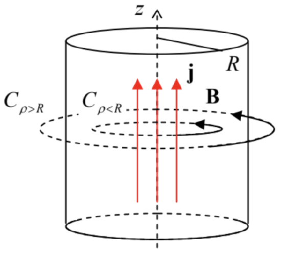Fig. 5.5. The simplest application of the Ampère law: the magnetic field of a straight current.

Selecting the Ampère-law contour \(\ C\) in the form of a ring of some radius \(\ \rho\) in the plane normal to the wire’s axis \(\ z\), we have \(\ \mathbf{B} \cdot d \mathbf{r}=B \rho d \varphi\), where \(\ \varphi\) is the azimuthal angle, so that Eq. (37) yields:

\[\ 2 \pi \rho B(\rho)=\mu_{0} \times \begin{cases}2 \pi \int_{0}^{\rho} j\left(\rho^{\prime}\right) \rho^{\prime} d \rho^{\prime}, & \text { for } \rho \leq R, \\ 2 \pi \int_{0}^{R} j\left(\rho^{\prime}\right) \rho^{\prime} d \rho^{\prime} \equiv I, & \text { for } \rho \geq R.\end{cases}\tag{5.38}\]

Thus we have not only recovered our previous result (20), with the notation replacement \(\ d \rightarrow \rho\), in a much simpler way, but could also find the magnetic field distribution inside the wire. In the most common case when the current is uniformly distributed along its cross-section, \(\ j(\rho)=\text { const }\), the first of Eqs. (38) immediately yields \(\ B \propto \rho\) for \(\ \rho \leq R\).

Another important system is a straight, long solenoid (Fig. 6a), with dense winding: \(\ n^{2} A >> 1\), where \(\ n\) is the number of wire turns per unit length, and \(\ A\) is the area of the solenoid’s cross-section.

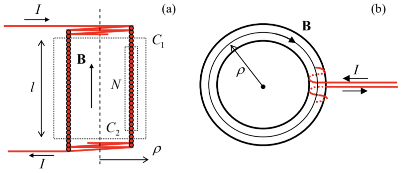Fig. 5.6. Calculating magnetic fields of (a) straight and (b) toroidal solenoids.

From the symmetry of this problem, the longitudinal (in Fig. 6a, vertical) component \(\ B_{z}\) of the magnetic field may only depend on the distance \(\ \rho\) of the observation point from the solenoid’s axis. First taking a plane Ampère contour \(\ C_{1}\), with both long sides outside the solenoid, we get \(\ B_{z}\left(\rho_{2}\right)-B_{z}\left(\rho_{1}\right)=0\), because the total current piercing the contour equals zero. This is only possible if \(\ B_{z}=0\) at any \(\ \rho\) outside of the solenoid, provided that it is infinitely long.¹⁷ With this result on hand, from the Ampère law applied to the contour \(\ C_{2}\), we get the following relation for the only (z-) component of the internal field:

\[\ B l=\mu_{0} N I,\tag{5.39}\]

where \(\ N\) is the number of wire turns passing through the contour of length \(\ l\). This means that regardless of the exact position of the internal side of the contour, the result is the same:

\[\ B=\mu_{0} \frac{N}{l} I \equiv \mu_{0} n I.\tag{5.40}\]

Thus, the field inside an infinitely long solenoid (with an arbitrary shape of its cross-section) is uniform; in this sense, a long solenoid is a magnetic analog of a wide plane capacitor, explaining why this system is so widely used in physical experiment.

As should be clear from its derivation, the obtained results, especially that the field outside of the solenoid equals zero, are conditional on the solenoid length being very large in comparison with its lateral size. (From Eq. (25), we may predict that for a solenoid of a finite length \(\ l\), the close-range external field is a factor of \(\ \sim A / l^{2}\) lower than the internal one.) Much better suppression of this “fringe” field may be obtained using the toroidal solenoid (Fig. 6b). The application of the Ampère law to this geometry shows that in the limit of dense winding \(\ (N >> 1)\), there is no fringe field at all (for any relation between two radii of the torus), while inside the solenoid, at distance \(\ \rho\) from the system’s axis,

\[\ B=\frac{\mu_{0} N I}{2 \pi \rho}.\tag{5.41}\]

We see that a possible drawback of this system for practical applications is that the internal field does depend on \(\ \rho\), i.e. is not quite uniform; however, if the torus is relatively thin, this deficiency is minor.

Next let us discuss a very important question: how can we solve the problems of magnetostatics for systems whose low symmetry does not allow getting easy results from the Ampère law? (The examples are of course too numerous to list; for example, we cannot use this approach even to reproduce Eq. (23) for a round current loop.) From the deep analogy with electrostatics, we may expect that in this case, we could calculate the magnetic field by solving a certain boundary problem for the field’s potential – in our current case, the vector potential \(\ \mathbf{A}\) defined by Eq. (28). However, despite the similarity of this formula and Eq. (1.38) for \(\ \phi\), which was noticed above, there are two additional issues we should tackle in the magnetic case.

First, calculating the vector potential distribution means determining three scalar functions (say, \(\ A_{x}, A_{y}\), and \(\ A_{z}\)), rather than one \(\ (\phi)\). To reveal the second, deeper issue, let us plug Eq. (27) into Eq. (35):

\[\ \nabla \times(\nabla \times \mathbf{A})=\mu_{0} \mathbf{j},\tag{5.42}\]

and then apply to the left-hand side of this equation the now-familiar identity (31). The result is

\[\ \nabla(\nabla \cdot \mathbf{A})-\nabla^{2} \mathbf{A}=\mu_{0} \mathbf{j}.\tag{5.43}\]

On the other hand, as we know from electrostatics (please compare Eqs. (1.38) and (1.41)), the vector potential \(\ \mathbf{A}(\mathbf{r})\) given by Eq. (28) has to satisfy a simpler (“vector-Poisson”) equation

\[\ \nabla^{2} \mathbf{A}=-\mu_{0} \mathbf{j},\quad\quad\quad\quad\text{Poisson equation for A}\tag{5.44}\]

which is just a set of three usual Poisson equations for each Cartesian component of \(\ \text { A }\).

To resolve the difference between these results, let us note that Eq. (43) is reduced to Eq. (44) if \(\ \nabla \cdot \mathbf{A}=0\). In this context, let us discuss what discretion do we have in the choice of the potential. In electrostatics, we might add to the scalar function \(\ \phi^{\prime}\) that satisfied Eq. (1.33) for the given field \(\ \mathbf{E}\), not only an arbitrary constant but even an arbitrary function of time:

\[\ -\nabla\left[\phi^{\prime}+f(t)\right]=-\nabla \phi^{\prime}=\mathbf{E}.\tag{5.45}\]

Similarly, using the fact that curl of the gradient of any scalar function equals zero,¹⁸ we may add to any vector function \(\ \mathbf{A}^{\prime}\) that satisfies Eq. (27) for the given field \(\ \mathbf{B}\), not only any constant but even a gradient of an arbitrary scalar function \(\ \chi(\mathbf{r}, t)\), because

\[\ \nabla \times\left(\mathbf{A}^{\prime}+\nabla \chi\right)=\nabla \times \mathbf{A}^{\prime}+\nabla \times(\nabla \chi)=\nabla \times \mathbf{A}^{\prime}=\mathbf{B}.\tag{5.46}\]

Such additions, which keep the fields intact, are called the gauge transformations.¹⁹ Let us see what such a transformation does to \(\ \nabla \cdot \mathbf{A^{\prime}}\):

\[\ \nabla \cdot\left(\mathbf{A}^{\prime}+\nabla \chi\right)=\nabla \cdot \mathbf{A}^{\prime}+\nabla^{2} \chi.\tag{5.47}\]

For any choice of such a function \(\ \mathbf{A}^{\prime}\), we can always choose the function \(\ \chi\) in such a way that it satisfies the Poisson equation \(\ \nabla^{2} \chi=-\nabla \cdot \mathbf{A}^{\prime}\), and hence makes the divergence of the transformed vector potential, \(\ \mathbf{A}=\mathbf{A}^{\prime}+\nabla \chi\), equal to zero everywhere,

\[\ \nabla \cdot \mathbf{A}=0,\quad\quad\quad\quad\text{Coulomb gauge}\tag{5.48}\]

thus reducing Eq. (43) to Eq. (44).

To summarize, the set of distributions \(\ \mathbf{A}^{\prime}(\mathbf{r})\) that satisfy Eq. (27) for a given field \(\ \mathbf{B}(\mathbf{r})\), is not limited to the vector potential \(\ \mathbf{A}(\mathbf{r})\) given by Eq. (44), but is reduced to it upon the additional Coulomb gauge condition (48). However, as we will see in a minute, even this condition still leaves some degrees of freedom in the choice of the vector potential. To illustrate this fact, and also to get a better gut feeling of the vector potential’s distribution in space, let us calculate \(\ \mathbf{A}(\mathbf{r})\) for two very basic cases.

First, let us revisit the straight wire problem shown in Fig. 5. As Eq. (28) shows, in this case the vector potential \(\ \mathbf{A}\) has just one component (along the axis \(\ z\)). Moreover, due to the problem’s axial symmetry, its magnitude may only depend on the distance from the axis: \(\ \mathbf{A}=\mathbf{n}_{z} A(\rho)\). Hence, the
gradient of \(\ \mathbf{A}\) is directed across the z-axis, so that Eq. (48) is satisfied at all points. For our symmetry \(\ (\partial / \partial \varphi=\partial / \partial z=0)\), the Laplace operator, written in cylindrical coordinates, has just one term,²⁰ reducing Eq. (44) to

\[\ \frac{1}{\rho} \frac{d}{d \rho}\left(\rho \frac{d A}{d \rho}\right)=-\mu_{0} j(\rho).\tag{5.49}\]

Multiplying both parts of this equation by \(\ \rho\) and integrating them over the coordinate once, we get

\[\ \rho \frac{d A}{d \rho}=-\mu_{0} \int_{0}^{\rho} j\left(\rho^{\prime}\right) \rho^{\prime} d \rho^{\prime}+\mathrm{const}.\tag{5.50}\]

Since in the cylindrical coordinates, for our symmetry, \(\ B=-d A / d \rho\),²¹ Eq. (50) is nothing else than our old result (38) for the magnetic field.²² However, let us continue the integration, at least for the region outside the wire, where the function \(\ A(\rho)\) depends only on the full current \(\ I\) rather than on the current distribution. Dividing both parts of Eq. (50) by \(\ \rho\), and integrating them over this argument again, we get

\[\ A(\rho)=-\frac{\mu_{0} I}{2 \pi} \ln \rho+\mathrm{const}, \quad \text { where } I=2 \pi \int_{0}^{R} j(\rho) \rho d \rho, \quad \text { for } \rho \geq R.\tag{5.51}\]

As a reminder, we had a similar logarithmic behavior for the electrostatic potential outside a uniformly charged straight line. This is natural because the Poisson equations for both cases are similar.

Now let us find the vector potential for the long solenoid (Fig. 6a), with its uniform magnetic field. Since Eq. (28) tells that the vector \(\ \mathbf{A}\) should follow the direction of the inducing current, we may start with looking for it in the form \(\ \mathbf{A}=\mathbf{n}_{\varphi} A(\rho)\). (This is especially natural if the solenoid’s cross-section is circular.) With this orientation of \(\ \mathbf{A}\), the same general expression for the curl operator in cylindrical coordinates yields \(\ \nabla \times \mathbf{A}=\mathbf{n}_{z}(1 / \rho) d(\rho A) / d \rho\). According to Eq. (27), this expression should be equal to \(\ \mathbf{B}\) – in our current case to \(\ \mathbf{n}_{z} B\), with a constant \(\ B\) – see Eq. (40). Integrating this equality, and selecting such integration constant that \(\ A(0)\) is finite, we get

\[\ A(\rho)=\frac{B\rho}{2},\quad\quad\quad\text { i.e. } \mathbf{A}=\frac{B \rho}{2} \mathbf{n}_{\varphi}.\tag{5.52}\]

Plugging this result into the general expression for the Laplace operator in the cylindrical coordinates,²³ we see that the Poisson equation (44) with \(\ \mathbf{j}=0\) (i.e. the Laplace equation), is satisfied again – which is natural since, for this distribution, the Coulomb gauge condition (48) is satisfied: \(\ \nabla \cdot \mathbf{A}=0\).

However, Eq. (52) is not the unique (or even the simplest) vector potential that gives the same uniform field \(\ \mathbf{B}=\mathbf{n}_{z} B\). Indeed, using the well-known expression for the curl operator in Cartesian coordinates,²⁴ it is straightforward to check that each of the vector functions \(\ \mathbf{A}^{\prime}=\mathbf{n}_{y} B x\) and \(\ \mathbf{A}^{\prime \prime}=-\mathbf{n}_{x} B y\) also has the same curl, and also satisfies the Coulomb gauge condition (48).²⁵ If such solutions do not look very natural because of their anisotropy in the [x, y] plane, please consider the fact that they represent the uniform magnetic field regardless of its source – for example, regardless of the shape of the long solenoid’s cross-section. Such choices of the vector potential may be very convenient for some problems, for example for the quantum-mechanical analysis of the 2D motion of a charged particle in the perpendicular magnetic field, giving the famous Landau energy levels.²⁶

---

Reference

¹² In the Gaussian units, Eq. (27) remains the same, and hence in Eq. (28), \(\ \mu_{0} / 4 \pi\) is replaced with \(\ 1 / c\).

¹³ See, e.g., MA Eq. (11.2).

¹⁴ See, E.g., MA Eq. (11.3).

¹⁵ As in all earlier formulas for the magnetic field, in the Gaussian units, the coefficient \(\ \mu_{0}\) in this relation is replaced with \(\ 4 \pi / c\).

¹⁶ See, e.g., MA Eq. (12.1) with \(\ \mathbf{f}=\mathbf{B}\).

¹⁷ Applying the Ampère law to a circular contour of radius \(\ \rho\), coaxial with the solenoid, we see that the field outside (but not inside!) it has an azimuthal component \(\ B_{\varphi}\), similar to that of the straight wire (see Eq. (38) above) and hence (at \(\ N >>1\)) much weaker than the longitudinal field inside the solenoid – see Eq. (40).

¹⁸ See, e.g., MA Eq. (11.1).

¹⁹ The use of the term “gauge” (originally meaning “a measure” or “a scale”) in this context is purely historic, so the reader should not try to find too much hidden sense in it.

²⁰ See, e.g., MA Eq. (10.3).

²¹ See, e.g., MA Eq. (10.5) with \(\ \partial / \partial \varphi=\partial / \partial z=0\).

²² Since the magnetic field at the wire’s axis has to be zero (otherwise, being normal to the axis, where would it be directed?), the integration constant in Eq. (50) has to equal zero.

²³ See, e.g., MA Eq. (10.6).

²⁴ See, e.g., MA Eq. (8.5).

²⁵ The axially-symmetric vector potential (52) is just a weighted sum of these two functions: \(\ \mathbf{A}=\left(\mathbf{A}^{\prime}+\mathbf{A}^{\prime \prime}\right) / 2\).

²⁶ See, e.g., QM Sec. 3.2.