9.2: Relativistic Kinematic Effects

Before proceeding to other corollaries of Eqs. (19), let us spend a few minutes discussing what do these relations actually mean. Evidently, they are trying to tell us that the spatial and temporal intervals are not absolute (as they are in the Newtonian space), but do depend on the reference frame they are measured in. So, we have to understand very clearly what exactly may be measured – and thus may be discussed in a meaningful physics theory. Recognizing this necessity, A. Einstein has introduced the notion of numerous imaginary observers that may be distributed all over each reference frame. Each observer has a clock and may use it to measure the instants of local events, taking take at their location. He also conjectured, very reasonably, that:

(i) all observers within the same reference frame may agree on a common length measure (“a scale”), i.e. on their relative positions in that frame, and synchronize their clocks,¹⁵ and

(ii) the observers belonging to different reference frames may agree on the nomenclature of world events (e.g., short flashes of light) to which their respective measurements refer.

Actually, these additional postulates have been already implied in our “derivation” of the Lorentz transform in Sec. 1. For example, by the set \(\ \{x, y, z, t\}\) we mean the results of space and time measurements of a certain world event, about that all observers belonging to frame 0 agree. Similarly, all observers of frame 0’ have to agree about the results \(\ \left\{x^{\prime}, y^{\prime}, z^{\prime}, t^{\prime}\right\}\). Finally, when the origin of frame 0’ passes by some sequential points xk of frame 0, observers in that frame may measure its passage times \(\ t_{k}\) without a fundamental error, and know that all these times belong to \(\ x^{\prime}=0\).

Now we can analyze the major corollaries of the Lorentz transform, which are rather striking from the point of view of our everyday (rather non-relativistic :-) experience.

(i) Length contraction. Let us consider a thin rigid rod, positioned along axis \(\ x\), with its length \(\ l \equiv x_2-x_1\), where \(\ x_{1,2}\) are the coordinates of the rod’s ends, as measured in its rest frame 0, at any instant \(\ t\) (Fig. 4). What would be the rod’s length \(\ l’\) measured by the Einstein observers in the moving frame 0’?

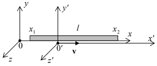Fig. 9.4. The relativistic length contraction.

At a time instant \(\ t^{\prime}\) agreed upon in advance, the observers who find themselves exactly at the rod’s ends, may register that fact, and then subtract their coordinates \(\ x_{1,2}^{\prime}\) to calculate the apparent rod length \(\ l^{\prime} \equiv x_{2}^{\prime}-x_{1}^{\prime}\) in the moving frame. According to Eq. (19a), \(\ l\) may be expressed via this \(\ l^{\prime}\) as

\[\ l \equiv x_{2}-x_{1}=\gamma\left(x_{2}^{\prime}+\beta c t^{\prime}\right)-\gamma\left(x_{1}^{\prime}+\beta c t^{\prime}\right)=\gamma\left(x_{2}^{\prime}-x_{1}^{\prime}\right) \equiv \gamma l^{\prime}.\tag{9.20a}\]

Hence, the rod’s length, as measured in the moving reference frame is

\[\ \text{Length contraction}\quad\quad\quad\quad l^{\prime}=\frac{l}{\gamma}=l\left(1-\frac{\nu^{2}}{c^{2}}\right)^{1 / 2} \leq l,\tag{9.20b}\]

in accordance with the FitzGerald-Lorentz hypothesis (5). This is the relativistic length contraction effect: an object is always the longest (has the so-called proper length \(\ l\)) if measured in its rest frame.

Note that according to Eqs. (19), the length contraction takes place only in the direction of the relative motion of two reference frames. As has been noted in Sec. 1, this result immediately explains the zero result of the Michelson-Morley-type experiments, so that they give very convincing evidence (if not irrefutable proof) of Eqs. (18)-(19).

(ii) Time dilation. Now let us use Eqs. (19a) to find the time interval \(\ \Delta t\), as measured in some reference frame 0, between two world events – say, two ticks of a clock moving with another frame 0’ (Fig. 5), i.e. having constant values of \(\ x^{\prime}, y^{\prime}\), and \(\ z^{\prime}\).

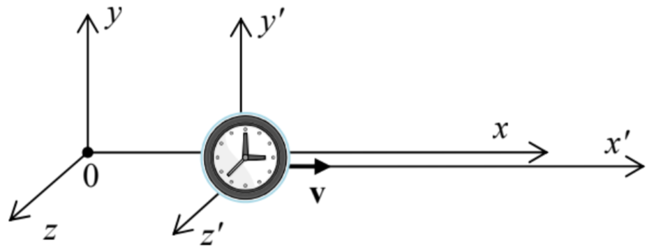Fig. 9.5. The relativistic time dilation.

Let the time interval between these two events, measured in the clock’s rest frame 0’, be \(\ \Delta t^{\prime} \equiv t_{2}^{\prime}-t_1^{\prime}\). At these two moments, the clock would fly by certain two Einstein’s observers at rest in the frame 0, so that they can record the corresponding moments \(\ t_{1,2}\) shown by their clocks, and then calculate \(\ \Delta t\) as their difference. According to the last of Eqs. (19a),

\[\ c \Delta t \equiv c t_{2}-c t_{1}=\gamma\left[\left(c t_{2}^{\prime}+\beta x^{\prime}\right)-\left(c t_{1}^{\prime}+\beta x^{\prime}\right)\right] \equiv \gamma c \Delta t^{\prime},\tag{9.21a}\]

so that, finally,

\[\ \Delta t=\gamma \Delta t^{\prime} \equiv \frac{\Delta t^{\prime}}{\left(1-\nu^{2} / c^{2}\right)^{1 / 2}} \geq \Delta t^{\prime}.\quad\quad\quad\quad\text{Time dilation}\tag{9.21b}\]

This is the famous relativistic time dilation (or “dilatation”) effect: a time interval is longer if measured in a frame (in our case, frame 0) moving relative to the clock, while that in the clock’s rest frame is the shortest possible – the so-called proper time interval.

This counter-intuitive effect is the everyday reality at experiments with high-energy elementary particles. For example, in a typical (and by no means record-breaking) experiment carried out in Fermilab, a beam of charged 200 GeV pions with \(\ \gamma \approx 1,400\) traveled a distance of \(\ l=300 \mathrm{~m}\) with the measured loss of only 3% of the initial beam intensity due to the pion decay (mostly, into muon-neutrino pairs) with the proper lifetime \(\ t_{0} \approx 2.56 \times 10^{-8} \mathrm{~s}\). Without the time dilation, only an \(\ \exp \left\{-l / c t_{0}\right\} \sim 10^{-17}\) fraction of the initial pions would survive, while the relativity-corrected number, \(\ \exp \{-l / c t\}=\exp \{-l/c\gamma t_0\}\approx0.97\), was in full accordance with experimental measurements.

As another example, the global positioning systems (say, the GPS) are designed with the account of the time dilation due to the velocity of their satellites (and also some gravity-induced, i.e. general-relativity corrections, which I would not have time to discuss) and would give large errors without such corrections. So, there is no doubt that time dilation (21) is a reality, though the precision of its experimental tests I am aware of¹⁶ has been limited by a few percent, because of the almost unavoidable involvement of less controllable gravity effects – which provide a time interval change of the opposite sign in most experiments near the Earth’s surface.

Before the first reliable observation of the time dilation (by B. Rossi and D. Hall in 1940), there had been serious doubts in the reality of this effect, the most famous being the twin paradox first posed (together with an immediate suggestion of its resolution) by P. Langevin in 1911. Let us send one of two twins on a long star journey with a speed \(\ \nu\) approaching \(\ c\). Upon his return to Earth, who of the twins would be older? The naïve approach is to say that due to the relativity principle, not one can be (and hence there is no time dilation) because each twin could claim that their counterpart rather than them, was moving, with the same speed but in the opposite direction. The resolution of the paradox in the general theory of relativity (which can handle not only the gravity, but also the acceleration effects) is that one of the twins had to be accelerated to be brought back, and hence the reference frames have to be dissimilar: only one of them may stay inertial all the time. Because of that, the twin who had been accelerated (“actually traveling”) would be younger than their sibling when they finally come together.

(iii) Velocity transformation. Now let us calculate the velocity \(\ \mathbf{u}\) of a particle, as observed in reference frame 0, provided that its velocity, as measured in frame 0’, is \(\ \mathbf{u}^{\prime}\) (Fig. 6).

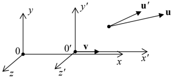Fig. 9.6. The relativistic velocity addition.

Keeping the usual definition of velocity, but with due attention to the relativity of not only spatial but also temporal intervals, we may write

\[\ \mathbf{u} \equiv \frac{d \mathbf{r}}{d t}, \quad \mathbf{u}^{\prime} \equiv \frac{d \mathbf{r}^{\prime}}{d t^{\prime}}.\tag{9.22}\]

Plugging in the differentials of the Lorentz transform relations (6a) into these definitions, we get

\[\ u_{x} \equiv \frac{d x}{d t}=\frac{d x^{\prime}+\nu d t^{\prime}}{d t^{\prime}+\nu d x^{\prime} / c^{2}} \equiv \frac{u_{x}^{\prime}+\nu}{1+u_{x}^{\prime} \nu / c^{2}}, \quad u_{y} \equiv \frac{d y}{d t}=\frac{1}{\gamma} \frac{d y^{\prime}}{d t^{\prime}+\nu d x^{\prime} / c^{2}} \equiv \frac{1}{\gamma} \frac{u_{y}^{\prime}}{1+u_{x}^{\prime} \nu / c^{2}},\tag{9.23}\]

and a similar formula for \(\ u_{z}\). In the classical limit \(\ \nu / c \rightarrow 0\), these relations are reduced to

\[\ u_{x}=u_{x}^{\prime}+\nu, \quad u_{y}=u_{y}^{\prime}, \quad u_{z}=u_{z}^{\prime},\tag{9.24a}\]

and may be merged into the familiar Galilean form

\[\ \mathbf{u}=\mathbf{u}^{\prime}+\mathbf{v}, \quad \text { for } \nu<<c.\tag{9.24b}\]

In order to see how unusual the full relativistic rules (23) are at \(\ u \sim c\), let us first consider a purely longitudinal motion, \(\ u_{y}=u_{z}=0\); then¹⁷

\[\ u=\frac{u^{\prime}+\nu}{1+u^{\prime} \nu / c^{2}},\quad\quad\quad\quad\text{Longitudinal velocity addition}\tag{9.25}\]

where \(\ u \equiv u_{x}\) and \(\ u^{\prime} \equiv u_{x}^{\prime}\). Figure 7 shows \(\ u\) as the function of \(\ u^{\prime}\) given by this formula, for several values of the reference frames’ relative velocity \(\ \nu\).

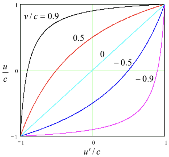Fig. 9.7. The addition of longitudinal velocities.

The first sanity check is that if \(\ \nu=0\), i.e. the reference frames are at rest relative to each other, then \(\ u=u^{\prime}\), as it should be – see the diagonal straight line in Fig. 7. Next, if magnitudes of \(\ u^{\prime}\) and \(\ \nu\) are both below \(\ c\), so is the magnitude of \(\ u\). (Also good, because otherwise ordinary particles in one frame would be tachyons in the other one, and the theory would be in big trouble.) Now strange things begin: even as \(\ u^{\prime}\) and \(\ \nu\) are both approaching \(\ c\), then \(\ u\) is also close to \(\ c\), but does not exceed it. As an example, if we fired forward a bullet with the relative speed \(\ 0.9 c\), from a spaceship moving from the Earth also at \(\ 0.9 c\), Eq. (25) predicts the speed of the bullet relative to Earth to be just \(\ [(0.9+0.9) /(1+0.9 \times 0.9)] c \approx 0.994c<c\), rather than \(\ (0.9+0.9) c=1.8 c>c\) as in the Galilean kinematics. Actually, we could expect this strangeness, because it is necessary to fulfill the 2^nd Einstein’s postulate: the independence of the speed of light in any reference frame. Indeed, for \(\ u^{\prime}=\pm c\), Eq. (25) yields \(\ u=\pm c\), regardless of \(\ \nu\).

In the opposite case of a purely transverse motion, when a particle moves across the relative motion of the frames (for example, at our choice of coordinates, \(\ u_{x}^{\prime}=u_{z}^{\prime}=0\), Eqs. (23) yield a much less spectacular result

\[\ u_{y}=\frac{u_{y}^{\prime}}{\gamma} \leq u_{y}^{\prime}.\tag{9.26}\]

This effect comes purely from the time dilation because the transverse coordinates are Lorentz-invariant.

In the case when both \(\ u_{x}^{\prime}\) and \(\ u_{y}^{\prime}\) are substantial (but \(\ u_{z}^{\prime}\) is still zero), we may divide Eqs. (23) by each other to relate the angles \(\ \theta\) of particle’s propagation, as observed in the two reference frames:

\[\ \tan \theta \equiv \frac{u_{y}}{u_{x}}=\frac{u_{y}^{\prime}}{\gamma\left(u_{x}^{\prime}+\nu\right)}=\frac{\sin \theta^{\prime}}{\gamma\left(\cos \theta^{\prime}+\nu / u^{\prime}\right)}\quad\quad\quad\quad\text{Stellar aberration effect}\tag{9.27}\]

This expression describes, in particular, the so-called stellar aberration effect: the dependence of the observed direction \(\ \theta\) toward a star on the speed v of the telescope’s motion relative to the star – see Fig. 8. (The effect is readily observable experimentally as the annual aberration due to the periodic change of speed \(\ \nu\) by \(\ 2 \nu_{\mathrm{E}} \approx 60 \mathrm{~km} / \mathrm{s}\) because of the Earth’s rotation about the Sun. Since the aberration’s main part is of the first order in \(\ \nu_{\mathrm{E}} / c \sim 10^{-4}\), this effect is very significant and has been known since the early 1700s.)

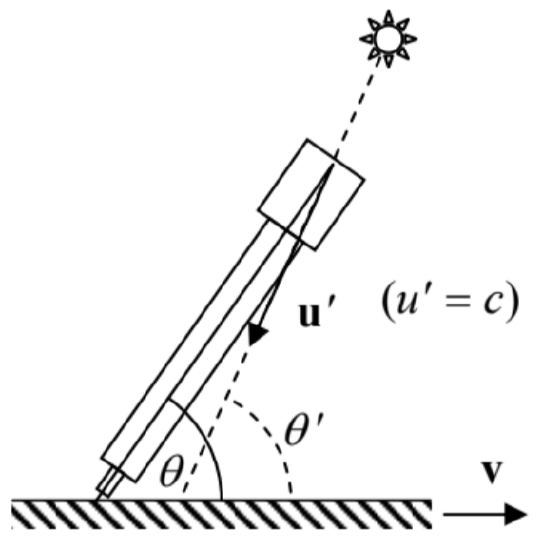Fig. 9.8. The stellar aberration.

For the analysis of this effect, it is sufficient to take, in Eq. (27), \(\ u^{\prime}=c\), i.e. \(\ \nu / u^{\prime}=\beta\), and interpret \(\ \theta^{\prime}\) as the “proper” direction to the star, that would be measured at \(\ \nu=0\).¹⁸ At \(\ \beta<<1\), both Eq. (27) and the Galilean result (which the reader is invited to derive directly from Fig. 8),

\[\ \tan \theta=\frac{\sin \theta^{\prime}}{\cos \theta^{\prime}+\beta}\tag{9.28}\]

may be well approximated by the first-order term

\[\ \Delta \theta \equiv \theta-\theta^{\prime} \approx-\beta \sin \theta^{\prime}.\tag{9.29}\]

Unfortunately, it is not easy to use the difference between Eqs. (27) and (28), of the second order in \(\ \beta\), for the special relativity confirmation, because other components of the Earth’s motion, such as its rotation, nutation, and torque-induced precession,¹⁹ give masking first-order contributions to the aberration.

Finally, for a completely arbitrary direction of vector \(\ \mathbf{u}^{\prime}\), Eqs. (22) may be readily used to calculate the velocity’s magnitude. The most popular form of the resulting expression is for the square of the relative velocity (or rather the reduced relative velocity \(\ \boldsymbol{\beta}\)) of two particles,

\[\ \beta^{2}=\frac{\left(\boldsymbol{\beta}_{1}-\boldsymbol{\beta}_{2}\right)^{2}-\left|\boldsymbol{\beta}_{1} \cdot \boldsymbol{\beta}_{2}\right|}{\left(1-\boldsymbol{\beta}_{1} \cdot \boldsymbol{\beta}_{2}\right)^{2}} \leq 1.\tag{9.30}\]

where \(\ \boldsymbol{\beta}_{1,2} \equiv \mathbf{v}_{1,2} / c\) are their normalized velocities as measured in the same reference frame.

(iv) The Doppler effect. Let us consider a monochromatic plane wave moving along the x-axis:

\[\ f=\operatorname{Re}\left[f_{\omega} \exp \{i(k x-\omega t\}] \equiv\left|f_{\omega}\right| \cos \left(k x-\omega t+\arg f_{\omega}\right) \equiv\left|f_{\omega}\right| \cos \Psi\right..\tag{9.31}\]

Its total phase, \(\ \Psi \equiv k x-\omega t+\arg f_{\omega}\) (in contrast to its amplitude \(\ \left|f_{\omega}\right|\) - see Sec. 5) cannot depend on the observer’s reference frame, because all fields of the wave vanish simultaneously at \(\ \Psi=\pi(n+1 / 2)\) (for all integer \(\ n\)), and such “world events” should be observable in all reference frames. The only way to keep \(\ \Psi=\Psi^{\prime}\) at all times is to have²⁰

\[\ k x-\omega t=k^{\prime} x^{\prime}-\omega^{\prime} t^{\prime}.\tag{9.32}\]

First, let us use this general relation to consider the Doppler effect in usual non-relativistic waves, e.g., oscillations of particles of a certain medium. Using the Galilean transform (2), we may rewrite Eq. (32) as

\[\ k\left(x^{\prime}+\nu t\right)-\omega t=k^{\prime} x^{\prime}-\omega^{\prime} t.\tag{9.32}\]

Since this transform leaves all space intervals (including the wavelength \(\ \lambda=2 \pi / k\)) intact, we can take \(\ k=k^{\prime}\), so that Eq. (33) yields

\[\ \omega^{\prime}=\omega-k \nu.\tag{9.34}\]

For a dispersion-free medium, the wave number \(\ k\) is the ratio of its frequency \(\ \omega\), as measured in the reference frame bound to the medium, and the wave velocity \(\ \nu_{\mathrm{w}}\). In particular, if the wave source rests in the medium, we may bind the reference frame 0 to the medium as well, and frame 0’ to the wave’s receiver (i.e. \(\ \nu=\nu_{\mathrm{r}}\)), so that

\[\ k=\frac{\omega}{\nu_{\mathrm{w}}},\tag{9.35}\]

and for the frequency perceived by the receiver, Eq. (34) yields

\[\ \omega^{\prime}=\omega \frac{\nu_{\mathrm{w}}-\nu_{\mathrm{r}}}{\nu_{\mathrm{w}}}.\tag{9.36}\]

On the other hand, if the receiver and the medium are at rest in the reference frame 0’, while the wave source is bound to the frame 0 (so that \(\ \nu=-\nu_{\mathrm{S}}\)), Eq. (35) should be replaced with

\[\ k=k^{\prime}=\frac{\omega^{\prime}}{\nu_{\mathrm{w}}},\tag{9.37}\]

and Eq. (34) yields a different result:

\[\ \omega^{\prime}=\omega \frac{\nu_{\mathrm{w}}}{\nu_{\mathrm{w}}-\nu_{\mathrm{s}}},\tag{9.38}\]

Finally, if both the source and detector are moving, it is straightforward to combine these two results to get the general relation

\[\ \omega^{\prime}=\omega \frac{\nu_{\mathrm{w}}-\nu_{\mathrm{r}}}{\nu_{\mathrm{w}}-\nu_{\mathrm{s}}}.\tag{9.39}\]

At low speeds of both the source and the receiver, this result simplifies,

\[\ \omega^{\prime} \approx \omega(1-\beta), \quad \text { with } \beta \equiv \frac{\nu_{\mathrm{r}}-\nu_{\mathrm{s}}}{\nu_{\mathrm{w}}},\tag{9.40}\]

but at speeds comparable to \(\ \nu_{\mathrm{w}}\) we have to use the more general Eq. (39). Thus, the usual Doppler effect is generally affected not only by the relative speed \(\ \left(\nu_{\mathrm{r}}-\nu_{\mathrm{s}}\right)\) of the wave’s source and detector but also of their speeds relative to the medium in which the waves propagate.

Somewhat counter-intuitively, for the electromagnetic waves the calculations are simpler because for them the propagation medium (aether) does not exist, the wave velocity equals \(\ \pm c\) in any reference frame, and there are no two separate cases: we can always take \(\ k=\pm \omega / c\) and \(\ k^{\prime}=\pm \omega^{\prime} / c\). Plugging these relations, together with the Lorentz transform (19a), into the phase-invariance condition (32), we get

\[\ \pm \frac{\omega}{c} \gamma\left(x^{\prime}+\beta c t^{\prime}\right)-\omega \gamma \frac{c t^{\prime}+\beta x^{\prime}}{c}=\pm \frac{\omega^{\prime}}{c} x^{\prime}-\omega^{\prime} t^{\prime}.\tag{9.41}\]

This relation has to hold for any \(\ x^{\prime}\) and \(\ t^{\prime}\), so we may require that the net coefficients before these variables vanish. These two requirements yield the same equality:

\[\ \omega^{\prime}=\omega \gamma(1 \mp \beta).\tag{9.42}\]

This result is already quite simple, but may be transformed further to be even more illuminating:

\[\ \omega^{\prime}=\omega \frac{1 \mp \beta}{\left(1-\beta^{2}\right)^{1 / 2}} \equiv \omega\left[\frac{(1 \mp \beta)(1 \mp \beta)}{(1+\beta)(1-\beta)}\right]^{1 / 2}.\tag{9.43}\]

At any sign before \(\ \beta\), one pair of parentheses cancel, so that²¹

\[\ \text{Longitudinal Doppler effect}\quad\quad\quad\quad \omega^{\prime}=\omega\left(\frac{1 \mp \beta}{1 \pm \beta}\right)^{1 / 2}.\tag{9.44}\]

Thus the Doppler effect for electromagnetic waves depends only on the relative velocity \(\ \nu=\beta c\) between the wave source and detector – as it should be, given the aether’s absence. At velocities much below c, Eq. (44) may be approximated as

\[\ \omega^{\prime} \approx \omega \frac{1 \mp \beta / 2}{1 \pm \beta / 2} \approx \omega(1 \mp \beta),\tag{9.45}\]

i.e. in the first approximation in \(\ \beta \equiv \nu / c\) it tends to the corresponding limit (40) of the usual Doppler effect.

If the wave vector k is tilted by angle \(\ \theta\) to the vector v (as measured in frame 0), then we have to repeat the calculations, with \(\ k\) replaced by \(\ k_{x}\), and components \(\ k_{y}\) and \(\ k_{z}\) left intact at the Lorentz transform. As a result, Eq. (42) is generalized as

\[\ \omega^{\prime}=\omega \gamma(1-\beta \cos \theta).\tag{9.46}\]

For the cases \(\ \cos \theta=\pm 1\), Eq. (46) reduces to our previous result (42). However, at \(\ \theta=\pi / 2\) (i.e. \(\ \cos \theta=0\)), the relation is rather different:

\[\ \omega^{\prime}=\gamma \omega \equiv \frac{\omega}{\left(1-\beta^{2}\right)^{1 / 2}}.\quad\quad\quad\quad \text{Transverse Doppler effect}\tag{9.47}\]

This is the transverse Doppler effect – which is absent in non-relativistic physics. Its first experimental evidence was obtained using electron beams (as had been suggested in 1906 by J. Stark), by H. Ives and G. Stilwell in 1938 and 1941. Later, similar experiments were repeated several times, but the first unambiguous measurements were performed only in 1979 by D. Hasselkamp et al. who confirmed Eq. (47) with a relative accuracy of about 10%. This precision may not look too spectacular, but besides the special tests discussed above, the Lorentz transform formulas have been also confirmed, less directly, by a huge body of other experimental data, especially in high energy physics, agreeing with calculations incorporating this transform as their part. This is why, with due respect to the spirit of challenging authority, I should warn the reader: if you decide to challenge the relativity theory (called “theory” by tradition only), you would also need to explain all these data. Best luck with that!²²

---

Reference

¹⁵ A posteriori, the Lorenz transform may be used to show that consensus-creating procedures (such as clock synchronization) are indeed possible. The basic idea of the proof is that at \(\ \nu<<c\), the relativistic corrections to space and time intervals are of the order of \(\ (\nu / c)^{2}\), they have negligible effects on clocks being brought together into the same point for synchronization slowly, with a speed \(\ u<<c\). The reader interested in a detailed discussion of this and other fine points of special relativity may be referred to, e.g., either H. Arzeliès, Relativistic Kinematics, Pergamon, 1966, or W. Rindler, Introduction to Special Relativity, 2^nd ed., Oxford U. Press, 1991.

¹⁶ See, e.g., J. Hafele and R. Keating, Science 177, 166 (1972).

¹⁷ With an account of the identity \(\ \tanh (a+b)=(\tanh a+\tanh b) /(1+\tanh a \tanh b)\), which readily follows from MA Eq. (3.5), Eq. (25) shows that that rapidities \(\ \varphi \equiv \tanh ^{-1} \beta\) add up exactly as longitudinal velocities at non-relativistic motion, making that notion very convenient for the analysis of transfer between several frames.

¹⁸ Strictly speaking, to reconcile the geometries shown in Fig. 1 (for which all our formulas, including Eq. (27), are valid) and Fig. 8 (giving the traditional scheme of the stellar aberration), it is necessary to invert the signs of \(\ \mathbf{u}\) (and hence \(\ \sin \theta^{\prime}\) and \(\ \cos \theta^{\prime}\)) and \(\ \mathbf{v}\), but as evident from Eq. (27), all the minus signs cancel, and the formula is valid as is.

¹⁹ See, e.g., CM Secs. 4.4-4.5.

²⁰ Strictly speaking, Eq. (32) is valid to an additive constant, but for notation simplicity, it may be always made equal to zero by selecting (at it has already been done in all relations of Sec. 1) the reference frame origins and/or clock turn-on times so that at \(\ t = 0\) and \(\ x = 0\), \(\ t^{\prime}=0\) and \(\ x^{\prime}=0\) as well.

²¹ It may look like the reciprocal expression of \(\ \omega\) via \(\ \omega^{\prime}\) is different, violating the relativity principle. However, in this case, we have to change the sign of \(\ \beta\), because the relative velocity of the system is opposite, so that we return to Eq. (44) again.

²² The same fact, ignored by crackpots, is also valid for other favorite directions of their attacks, including the Universe expansion, quantum measurement uncertainty, and entropy growth in physics, and the evolution theory in biology.