
9.6: Relativistic Particles in Electric and Magnetic Fields


- Last updated
- Mar 5, 2022
- Save as PDF

( \newcommand{\kernel}{\mathrm{null}\,}\)
Now let us analyze the dynamics of charged particles in electric and magnetic fields. Inspired by “our” success in forming the 4-vector (75) of the energy-momentum, with the contravariant form
pα={Ec,p}=γ{mc,p}=mdxαdτ≡muα,
where uα is the contravariant form of the 4-velocity (63) of the particle,
uα≡dxαdτ,uα≡dxαdτ,
we may notice that the non-relativistic equation of motion, resulting from the Lorentz-force formula (5.10) for the three spatial components of pa, at charged particle’s motion in an electromagnetic field,
Particle’s equation of motiondpdt=q(E+u×B),
is fully consistent with the following 4-vector equality (which is evidently form-invariant with respect to the Lorentz transform):
Particle’s dynamics: 4-formdpαdτ=qFαβuβ.
For example, according to Eq. (125), the α=1 component of this equation reads
dp1dτ=qF1βuβ=q[Excγc+0⋅(−γux)+(−Bz)(−γuy)+By(−μuz)]=qγ[E+u×B]x,
and similarly for two other spatial components ( α=2 and α=3). It may look that these expressions differ from the 2nd Newton law (144) by the extra factor γ. However, plugging into Eq. (146) the definition of the proper time interval, dτ=dt/γ, and canceling γ in both parts, we recover Eq. (144) exactly – for any velocity of the particle! The only caveat is that if u is comparable with c, the vector p in Eq. (144) has to be understood as the relativistic momentum (70), proportional to the velocity-dependent mass M=γm≥m rather than to the rest mass m.
The only remaining general task is to examine the meaning of the 0th component of Eq. (145). Let us spell it out:
dp0dτ=qF0βuβ=q[0⋅γc+(−Exc)(−γux)+(−Eyc)(−γuy)+(−Ezc)(−γuz)]=qγEc⋅u.
Recalling that p0=E/c, and using the basic relation dτ=dt/γ again, we see that Eq. (147) looks exactly as the non-relativistic relation for the kinetic energy change (what is sometimes called the work-energy principle, in our case for the Lorentz force only54):
dEdt=qE⋅u,Particle’s energy: evolution
besides that in the relativistic case, the energy has to be taken in the general form (73).
No question, the 4-component equation (145) of the relativistic dynamics is absolutely beautiful in its simplicity. However, for the solution of particular problems, Eqs. (144) and (148) are frequently more convenient. As an illustration of this point, let us now use these equations to explore relativistic effects at charged particle motion in uniform, time independent electric and magnetic fields. In doing that, we will, for the time being, neglect the contributions into the field by the particle itself.55
(i) Uniform magnetic field. Let the magnetic field be constant and uniform in the “lab” reference frame 0. Then in this frame, Eqs. (144) and (148) yield
dpdt=qu×B,dEdt=0.
From the second equation, E=const, we get u= const ,β≡u/c= const ,γ≡(1−β2)−1/2= const , and M≡γm= const, so that the first of Eqs. (149) may be rewritten as
dudt=u×ωc,
where ωc is the vector directed along the magnetic field B, with the magnitude equal to the following cyclotron frequency (sometimes called “gyrofrequency”):
ωc≡qBM=qBγm=qc2BE.Cyclotron frequency
If the particle’s initial velocity u0 is perpendicular to the magnetic field, Eq. (150) describes its circular motion, with a constant speed u=u0, in a plane perpendicular to B, with the angular velocity (151). In the non-relativistic limit u<<c, when γ→1, i.e. M→m, the cyclotron frequency ωc equals qB/m, i.e. is independent of the speed. However, as the kinetic energy of the particle is increased to become comparable with its rest energy mc2, the frequency decreases, and in the ultra-relativistic limit:
ωc≈qcBp<<qBm, for u≈c.
The cyclotron motion’s radius may be calculated as R=u/ωc; in the non-relativistic limit it is proportional to the particle’s speed, i.e. to the square root of its kinetic energy. However, as Eq. (151) shows, in the general case the radius is proportional to the particle’s relativistic momentum rather than its speed:
R=uωc=MuqB=mγuqB=1qpB,Cyclotron radius
so that in the ultra-relativistic limit, when p≈E/c, R is proportional to the kinetic energy.
These dependences of ωc and R on energy are the major factors in the design of circular accelerators of charged particles. In the simplest of these machines (the cyclotron, invented in 1929 by Ernest Orlando Lawrence), the frequency ω of the accelerating ac electric field is constant, so that even it is tuned to the ωc of the initially injected particles, the drop of the cyclotron frequency with energy eventually violates this tuning. Due to this reason, the largest achievable particle’s speed is limited to just ∼0.1 c (for protons, corresponding to the kinetic energy of just ∼15 MeV). This problem may be addressed in several ways. In particular, in synchrotrons (such as Fermilab’s Tevatron and the CERN’s Large Hadron Collider, LHC56) the magnetic field is gradually increased in time to compensate for the momentum increase (B∝p), so that both R (148) and ωc (147) stay constant, enabling proton acceleration to energies as high as ∼7 TeV, i.e. ∼2,000 mc2.57
Returning to our initial problem, if the particle’s initial velocity has a component u‖ along the magnetic field, then it is conserved in time, so that the trajectory is a spiral around the magnetic field lines. As Eqs. (149) show, in this case Eq. (150) remains valid, but in Eqs. (151) and (153) the full speed and momentum have to be replaced with magnitudes of their (also time-conserved) components, u⊥ and p⊥, normal to B, while the Lorentz factor γ in those formulas still includes the full speed of the particle.
Finally, in the special case when the particle’s initial velocity is directed exactly along the magnetic field’s direction, it continues to move by straight line along the vector B. In this case, the cyclotron frequency still has its non-zero value (151) but does not correspond to any real motion, because R=0.
(ii) Uniform electric field. This problem is (technically) more complex than the previous one, because in the electric field, the particle’s energy changes. Directing the z-axis along the field E, from Eq. (144) we get
dpzdt=qE,dp⊥dt=0.
If the field does not change in time, the first integration of these equations is elementary,
pz(t)=pz(0)+qEt,p⊥(t)=const=p⊥(0),
but the further integration requires care, because the effective mass M=γm of the particle depends on its full speed u, with
u2=u2z+u2⊥,
making the two motions, along and across the field, mutually dependent.
If the initial velocity is perpendicular to the field E, i.e. if pz(0)=0,p⊥(0)=p(0)≡p0, the easiest way to proceed is to calculate the kinetic energy first:
E2=(mc2)2+c2p2(t)≡E20+c2(qEt)2, where E0≡[(mc2)2+c2p20]1/2.
On the other hand, we can calculate the same energy by integrating Eq. (148),
dEdt=qE⋅u≡qEdzdt,
over time, with a simple result:
E=E0+qEz(t),
where (just for the notation simplicity) I took z(0)=0. Requiring Eq. (159) to give the same E2 as Eq. (157), we get a quadratic equation for the function z(t),
E20+c2(qEt)2=[E0+qEz(t)]2,
whose solution (with the sign before the square root corresponding to E>0, i.e. to z≥0) is
z(t)=E0qE{[1+(cqEtE0)2]1/2−1}.
Now let us find the particle’s trajectory. Selecting the x-axis so that the initial velocity vector (and hence the velocity vector at any further instant) is within the [x,z] plane, i.e. that y(t)=0 identically, we may use Eqs. (155) to calculate the trajectory’s slope, at its arbitrary point, as
dzdx≡dz/dtdx/dt≡MuzMux≡pzpx=qEtp0.
Now let us use Eq. (160) to express the numerator of this fraction, qEt, as a function of z:
qEt=1c[(E0+qEz)2−E20]1/2.
Plugging this expression into Eq. (161), we get
dzdx=1cp0[(E0+qEz)2−E20]1/2.
This differential equation may be readily integrated separating the variables z and x, and using the following substitution: ξ≡cosh−1(qEz/ε0+1). Selecting the origin of axis x at the initial point, so that x(0)=0, we finally get the trajectory:
z=E0qE(coshqExcp0−1).
This curve is usually called the catenary, but sometimes the “chainette”, because it (with the proper constant replacement) describes the stationary shape of a heavy, uniform chain in a uniform gravity field, directed along the z-axis. At the initial part of the trajectory, where qEx<cp0(0), this expression may be approximated with the first non-zero term of its Taylor expansion in small x, giving the following parabola:
z=E0qE2(xcp0)2,
so that if the initial velocity of the particle is much less than c (i.e. p0≈mu0,E0≈mc2), we get the very familiar non-relativistic formula:
z=qE2mu20x2≡a2t2, with a=Fm=qEm.
The generalization of this solution to the case of an arbitrary direction of the particle’s initial velocity is left for the reader’s exercise.
(iii) Crossed uniform magnetic and electric fields (E⊥B). In the view of the somewhat bulky solution of the previous problem (i.e. the particular case of the current problem for B=0), one might think that this problem, with B≠0, should be forbiddingly complex for an analytical solution. Counter-intuitively, this is not the case, due to the help from the field transform relations (135). Let us consider two possible cases.
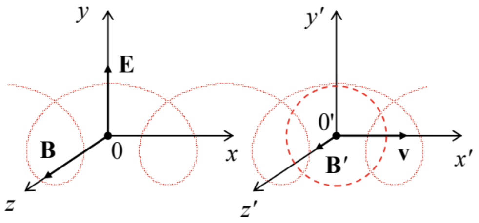
Case 1: E/c<B. Let us consider an inertial reference frame 0’ moving (relatively the “lab” reference frame 0 in which the fields E and B are defined) with the following velocity:
v=E×BB2,
and hence the magnitude ν=c×(E/c)/B<c. Selecting the coordinate axes as shown in Fig. 12, so that
Ex=0,Ey=E,Ez=0;Bx=0,By=0,Bz=0,
we see that the Cartesian components of this velocity are νx=ν,νy=νz=0.
Since this choice of the coordinates complies with the one used to derive Eqs. (134), we can readily use that simple form of the Lorentz transform to calculate the field components in the moving reference frame:
E′x=0,E′y=γ(E−νB)≡γ(E−EBB)≡0,E′z=0,
B′x=0,B′y=0,B′z=γ(B−νEc2)≡γB(1−νEBc2)≡γB(1−ν2c2)≡Bγ≤B,
where the Lorentz parameter γ≡(1−ν2/c2)−1/2 corresponds to the velocity (168) rather than that of the particle. These relations show that in this special reference frame the particle only “sees” the re-normalized uniform magnetic field B′≤B, parallel to the initial field, i.e. perpendicular to the velocity (168). Using the result of the above case (i), we see that in this frame the particle moves along either a circle or a spiral winding about the direction of the magnetic field, with the angular velocity (151):
ω′c=qB′E′/c2,
and the radius (153):
R′=p′⊥qB′.
Hence in the lab frame, the particle performs this orbital/spiral motion plus a “drift” with the constant velocity v (Fig. 12). As the result, the lab-frame trajectory of the particle (or rater its projection onto the plane normal to the magnetic field) is a trochoid-like curve58 that, depending on the initial velocity, may be either prolate (self-crossing), as in Fig. 12, or curtate (drift-stretched so much that it is not self-crossing).
Such looped motion of electrons is used, in particular, in magnetrons – very popular generators of microwave radiation. In such a device (Fig. 13), the magnetic field, usually created by specially-shaped permanent magnets, is nearly uniform (in the region of electron motion) and directed along the magnetron’s axis (in Fig. 13, normal to the plane of the drawing), while the electric field of magnitude E<<cB, created by the dc voltage applied between the anode and cathode, is virtually radial.
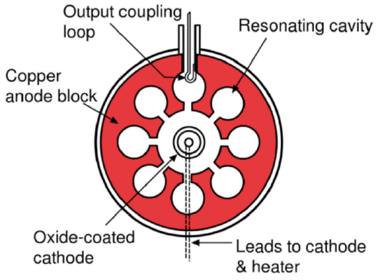 Fig. 9.13. Schematic cross-section of a typical magnetron. (Figure adapted from https://en.Wikipedia.org/wiki/Cavity_magnetron under the Free GNU Documentation License.)
As a result, the above simple theory is only approximately valid, and the electron trajectories are close to epicycloids rather than trochoids. The applied electric field is adjusted so that these looped trajectories pass close to the anode’s surface, and hence to the gap openings of the cylindrical microwave cavities drilled in the anode’s bulk. The fundamental mode of such a cavity is quasi-lumped, with the cylindrical walls working mostly as inductances, and the gap openings as capacitances, with the microwave electric field concentrated in these openings. This is why the mode is strongly coupled to the electrons passing nearby, and their interaction creates large positive feedback (equivalent to negative damping), which results in intensive microwave self-oscillations at the cavities’ own frequency.59 The oscillation energy, of course, is taken from the dc-field-accelerated electrons; due to their energy loss, the looped trajectory of each electron gradually moves closer to the anode and finally lands on its surface. The wide use of such generators (in particular, in microwave ovens, which operate in a narrow frequency band around 2.45 GHz, allocated for these devices to avoid their interference with wireless communication systems) is due to their simplicity and high (up to 65%) efficiency.
Case 2: E/c>B. In this case, the speed given by Eq. (168) would be above the speed of light, so let us introduce a reference frame moving with a different velocity,
v=E×B(E/c)2,
whose direction is the same as before (Fig. 12), and magnitude ν=c×B/(E/c) is again below c. A calculation absolutely similar to the one performed above for Case 1, yields
E′x=0,E′y=γ(E−νB)=γE(1−νBE)=γE(1−ν2c2)=Eγ≤E,E′z=0,
B′x=0,B′y=0,B′z=γ(B−νEc2)=γ(B−EBE)=0.
so that in the moving frame the particle “sees” only the electric field E′≤E. According to the solution of our previous problem (ii), the trajectory of the particle in the moving frame is the catenary (165), so that in the lab frame it has an “open”, hyperbolic character as well.
To conclude this section, let me note that if the electric and magnetic fields are nonuniform, the particle motion may be much more complex, and in most cases, the integration of equations (144), (148) may be carried out only numerically. However, if the field’s nonuniformity is small, approximate analytical methods may be very effective. For example, if E=0, and the magnetic field has a small transverse gradient ∇B in a direction normal to the vector B itself, such that
η≡|∇B|B<<1R,
where R is the cyclotron radius (153), then it is straightforward to use Eq. (150) to show60 that the cyclotron orbit drifts perpendicular to both B and ∇B, with the drift speed
νd≈ηωc(12u2⊥+u2‖)<<u.
The physics of this drift is rather simple: according to Eq. (153), the instant curvature of the cyclotron orbit is proportional to the local value of the field. Hence if the field is nonuniform, the trajectory bends slightly more on its parts passing through a stronger field, thus acquiring a shape close to a curate trochoid.
For experimental physics and engineering practice, the effects of longitudinal gradients of magnetic field on the charged particle motion are much more important, but it is more convenient for me to postpone their discussion until we have developed a little bit more analytical tools in the next section.
Reference
54 See, e.g., CM Eq. (1.20) divided by dt, and with dp/dt=F=qE. (As a reminder, the magnetic field cannot affect the particle’s energy, because the magnetic component of the Lorentz force is perpendicular to its velocity.)
55 As was emphasized earlier in this course, in statics this contribution has to be ignored. In dynamics, this is generally not true; these self-action effects (which are, in most cases, negligible) will be discussed in the next chapter.
56 See https://home.cern/topics/large-hadron-collider.
57 For more on this topic, I have to refer the interested reader to special literature, for example, either S. Lee, Accelerator Physics, 2nd ed., World Scientific, 2004, or E. Wilson, An Introduction to Particle Accelerators, Oxford U. Press, 2001.
58 As a reminder, a trochoid may be described as the trajectory of a point on a rigid disk rolled along a straight line. It’s canonical parametric representation is x=Θ+acosΘ,y=asinΘ. (For a>1, the trochoid is prolate, if a<1, it is curtate, and if a=1, it is called the cycloid.) Note, however, that for our problem, the trajectory in the lab frame is exactly trochoidal only in the non-relativistic limit ν<<c (i.e. E/c<<B).
59 See, e.g., CM Sec. 5.4.
60 See, e.g., Sec. 12.4 in J. Jackson, Classical Electrodynamics, 3rd ed., Wiley, 1999.