9.3: 4-vectors, Momentum, Mass, and Energy

Before proceeding to the relativistic dynamics, let us discuss the mathematical formalism that makes all the calculations more compact – and more beautiful. We have already seen that the three spatial coordinates \(\ \{x, y, z\}\) and the product \(\ ct\) are Lorentz-transformed similarly – see Eqs. (18)-(19) again. So it is natural to consider them as components of a single four-component vector (or, for short, 4-vector),

\[\ \left\{x_{0}, x_{1}, x_{2}, x_{3}\right\} \equiv\{c t, \mathbf{r}\},\tag{9.48}\]

with components

\[\ x_{0} \equiv c t, \quad x_{1} \equiv x, \quad x_{2} \equiv y, \quad x_{3} \equiv z.\quad\quad\quad\quad\text{Space-time 4-vector}\tag{9.49}\]

According to Eqs. (19), its components are Lorentz-transformed as

\[\ x_{j}=\sum_{j^{\prime}=0}^{3} L_{j j^{\prime}} x_{j^{\prime}}^{\prime},\quad\quad\quad\quad\text{Lorentz transform: 4-form}\tag{9.50}\]

where \(\ L_{j j^{\prime}}\) are the elements of the following \(\ 4 \times 4\) Lorentz transform matrix

\[\ \left(\begin{array}{cccc}
\gamma & \beta \gamma & 0 & 0 \\
\beta \gamma & \gamma & 0 & 0 \\
0 & 0 & 1 & 0 \\
0 & 0 & 0 & 1
\end{array}\right).\quad\quad\quad\quad \text{Lorentz transform matrix}\tag{9.51}\]

Since such 4-vectors are a new notion for this course and will be used for many more purposes than just the space-time transform, we need to discuss the general mathematical rules they obey. Indeed, as was already mentioned in Sec. 8.9, the usual (three-component) vector is not just any ordered set (string) of three scalars \(\ \left\{A_{x}, A_{y}, A_{z}\right\}\); if we want it to represent a reference-frame-independent physical reality, the vector’s components have to obey certain rules at the transfer from one reference frame to another. In particular, in the non-relativistic limit the vector’s norm (its magnitude squared),

\[\ A^{2}=A_{x}^{2}+A_{y}^{2}+A_{z}^{2},\tag{9.52}\]

should be invariant with respect to the transfer between different reference frames. However, a naïve extension of this approach to 4-vectors would not work, because, according to the calculations of Sec. 1, the Lorentz transform keeps intact the combinations of the type (7), with one sign negative, rather than the sum of all components squared. Hence for the 4-vectors, all the rules of the game have to be reviewed and adjusted – or rather redefined from the very beginning.

An arbitrary 4-vector is a string of 4 scalars,²³

\[\ \text{General 4-vector}\quad\quad\quad\quad \left\{A_{0}, A_{1}, A_{2}, A_{3}\right\},\tag{9.53}\]

whose components \(\ A_{j}\), as measured in the systems 0 and 0’ shown in Fig. 1, obey the Lorentz transform relations similar to Eq. (50):

\[\ \text{Lorentz transform: general 4-vector}\quad\quad\quad\quad A_{j}=\sum_{j^{\prime}=0}^{3} L_{j j^{\prime}} A_{j^{\prime}}^{\prime}.\tag{9.54}\]

As we have already seen on the example of the space-time 4-vector (48), this means in particular that

\[\ \text{Lorentz invariance}\quad\quad\quad\quad A_{0}^{2}-\sum_{j=1}^{3} A_{j}^{2}=\left(A_{0}^{\prime}\right)^{2}-\sum_{j=1}^{3}\left(A_{j}^{\prime}\right)^{2}.\tag{9.55}\]

This is the so-called Lorentz invariance condition for the 4-vector’s norm. (The difference between this relation and Eq. (52), pertaining to the Euclidian geometry, is the reason why the Minkowski space is called pseudo-Euclidian.) It is also straightforward to use Eqs. (51) and (54) to check that an evident generalization of the norm, the scalar product of two arbitrary 4-vectors,

\[\ \text{Scalar 4-product}\quad\quad\quad\quad A_{0} B_{0}-\sum_{j=1}^{3} A_{j} B_{j},\tag{9.56}\]

is also Lorentz-invariant.

Now consider the 4-vector corresponding to a small interval between two close world events:

\[\ \left\{d x_{0}, d x_{1}, d x_{2}, d x_{3}\right\}=\{c d t, d \mathbf{r}\};\tag{9.57}\]

its norm,

\[\ \text{Interval}\quad\quad\quad\quad (d s)^{2} \equiv d x_{0}^{2}-\sum_{j=1}^{3} d x_{j}^{2}=c^{2}(d t)^{2}-(d r)^{2},\tag{9.58}\]

is of course also Lorentz-invariant. Since the speed of any particle (or signal) cannot be larger than \(\ c\), for any pair of world events that are in a causal relation with each other, \(\ (d r)^{2}\) cannot be larger than \(\ (c d t)^{2}\), i.e. such time-like interval \(\ (d s)^{2}\) cannot be negative. The 4D surface separating such intervals from space-like intervals \(\ (d s)^{2}<0\) is called the light cone (Fig. 9).

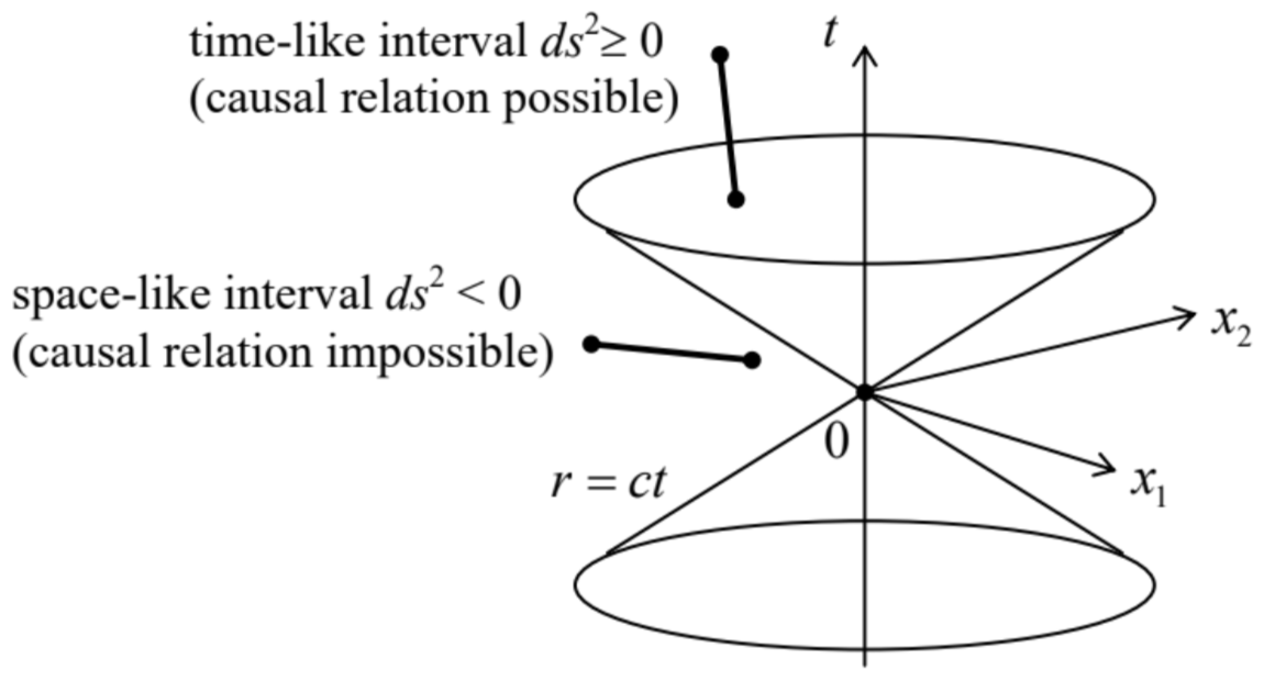Fig. 9.9. A 2+1 dimensional image of the light cone – which is actually 3+1 dimensional.

Now let us assume that two close world events happen with the same particle that moves with velocity u. Then in the frame moving with the particle (v = u), on the right-hand side of Eq. (58) the last term equals zero, while the involved time is the proper one, so that

\[\ d s=c d \tau,\tag{9.59}\]

where \(\ d \tau\) is the proper time interval. But according to Eq. (21), this means that we can write

\[\ d \tau=\frac{d t}{\gamma},\tag{9.60}\]

where \(\ dt\) is the time interval in an arbitrary (besides being inertial) reference frame, while

\[\ \boldsymbol{\beta} \equiv \frac{\mathbf{u}}{c} \quad \text { and } \gamma \equiv \frac{1}{\left(1-\beta^{2}\right)^{1 / 2}}=\frac{1}{\left(1-u^{2} / c^{2}\right)^{1 / 2}}\tag{9.61}\]

are the parameters (17) corresponding to the particle’s velocity (\(\ \mathbf{u}\)) in that frame, so that \(\ d s=c d t / \gamma\).²⁴

Let us use Eq. (60) to explore whether a 4-vector may be formed using the spatial components of the particle’s velocity

\[\ \mathbf{u}=\left\{\frac{d x}{d t}, \frac{d y}{d t}, \frac{d z}{d t}\right\}.\tag{9.62}\]

Here we have a slight problem: as Eqs. (22) show, these components do not obey the Lorentz transform. However, let us use \(\ d \tau \equiv d t / \gamma\), the proper time interval of the particle, to form the following string:

\[\ \left\{\frac{d x_{0}}{d \tau}, \frac{d x_{1}}{d \tau}, \frac{d x_{2}}{d \tau}, \frac{d x_{3}}{d \tau}\right\} \equiv \gamma\left\{c, \frac{d x}{d t}, \frac{d y}{d t}, \frac{d z}{d t}\right\} \equiv \gamma\{c, \mathbf{u}\}.\quad\quad\quad\quad\text{4-velocity}\tag{9.63}\]

As it follows from the comparison of the middle form of this expression with Eq. (48), since the time-space vector obeys the Lorentz transform, and \(\ \tau\) is Lorentz invariant, the string (63) is a legitimate 4-vector; it is called the 4-velocity of the particle.

Now we are well equipped to proceed to relativistic dynamics. Let us start with such basic notions as the momentum \(\ \mathbf{p}\) and the energy \(\ \mathscr{E}\)-so far, for a free particle.²⁵ Perhaps the most elegant way to “derive” (or rather guess²⁶) the expressions for \(\ \mathbf{p}\) and \(\ \mathscr{E}\) as functions of the particle’s velocity \(\ \mathbf{u}\), is based on analytical mechanics. Due to the conservation of \(\ \mathbf{v}\), the trajectory of a free particle in the 4D Minkowski space \(\ \{c t, \mathbf{r}\}\) is always a straight line. Hence, from the Hamilton principle,²⁷ we may expect its action \(\ \mathscr{S}\), between points 1 and 2, to be a linear function of the space-time interval (59):

\[\ \text{Free particle: action}\quad\quad\quad\quad \mathscr{S}=\alpha \int_{1}^{2} d s \equiv \alpha c \int_{1}^{2} d \tau \equiv \alpha c \int_{t_{1}}^{t_{2}} \frac{d t}{\gamma},\tag{9.64}\]

where \(\ \alpha\) is some constant. On the other hand, in analytical mechanics, the action is defined as

\[\ \mathscr{S} \equiv \int_{t_{1}}^{t_{2}} \mathscr{L} d t,\tag{9.65}\]

where \(\ \mathscr{L}\) is particle’s Lagrangian function.²⁸ Comparing these two expressions, we get

\[\ \mathscr{L}=\frac{\alpha c}{\gamma} \equiv \alpha c\left(1-\frac{u^{2}}{c^{2}}\right)^{1 / 2}.\tag{9.66}\]

In the non-relativistic limit \(\ (u<<c)\), this function tends to

\[\ \mathscr{L} \approx \alpha c\left(1-\frac{u^{2}}{2 c^{2}}\right)=\alpha c-\frac{\alpha u^{2}}{2 c}.\tag{9.67}\]

To correspond to the Newtonian mechanics,²⁹ the last (velocity-dependent) term should equal \(\ m u^{2} / 2\). From here we find \(\ \alpha=-m c\), so that, finally,

\[\ \text{Free particle: Lagrangian function}\quad\quad\quad\quad \mathscr{L}=-m c^{2}\left(1-\frac{u^{2}}{c^{2}}\right)^{1 / 2} \equiv-\frac{m c^{2}}{\gamma}.\tag{9.68}\]

Now we can find the Cartesian components \(\ p_{j}\) of the particle’s momentum as the generalized momenta corresponding to the corresponding components \(\ r_{j}(j=1,2,3)\) of the 3D radius-vector \(\ \mathbf{r}\):³⁰

\[\ p_{j}=\frac{\partial \mathscr{L}}{\partial \dot{r}_{j}} \equiv \frac{\partial \mathscr{L}}{\partial u_{j}}=-m c^{2} \frac{\partial}{\partial u_{j}}\left(1-\frac{u_{1}^{2}+u_{2}^{2}+u_{3}^{2}}{c^{2}}\right)^{1 / 2}=\frac{m u_{j}}{\left(1-u^{2} / c^{2}\right)^{1 / 2}} \equiv m \gamma u_{j}.\tag{9.69}\]

Thus for the 3D vector of momentum, we can write the result in the same form as in non-relativistic mechanics,

\[\ \mathbf{p}=m \gamma \mathbf{u} \equiv M \mathbf{u},\quad\quad\quad\quad \text{Relativistic momentum}\tag{9.70}\]

using the reference-frame-dependent scalar \(\ M\) (called the relativistic mass) defined as

\[\ M \equiv m \gamma=\frac{m}{\left(1-u^{2} / c^{2}\right)^{1 / 2}} \geq m,\quad\quad\quad\quad\text{Relativistic mass}\tag{9.71}\]

\(\ m\) being the non-relativistic mass of the particle. (More often, m is called the rest mass, because in the reference frame in that the particle rests, Eq. (71) yields \(\ M = m\).)

Next, let us return to analytical mechanics to calculate the particle’s energy \(\ \mathscr{E}\) (which for a free particle coincides with its Hamiltonian function \(\ \mathscr{H}\)):³¹

\[\ \mathscr{E}=\mathscr{H}=\sum_{j=1}^{3} p_{j} u_{j}-\mathscr{L}=\mathbf{p} \cdot \mathbf{u}-\mathscr{L}=\frac{m u^{2}}{\left(1-u^{2} / c^{2}\right)^{1 / 2}}+m c^{2}\left(1-\frac{u^{2}}{c^{2}}\right)^{1 / 2} \equiv \frac{m c^{2}}{\left(1-u^{2} / c^{2}\right)^{1 / 2}}.\quad\quad\quad\quad \mathscr{E}=Mc^2\tag{9.73}\]

which expresses the relation between the free particle’s mass and its energy.³² In the non-relativistic limit, it reduces to

\[\ \mathscr{E}=\frac{m c^{2}}{\left(1-u^{2} / c^{2}\right)^{1 / 2}} \approx m c^{2}\left(1+\frac{u^{2}}{2 c^{2}}\right)=m c^{2}+\frac{m u^{2}}{2},\tag{9.74}\]

the first term \(\ m c^{2}\) being called the rest energy of a particle.

Now let us consider the following string of 4 scalars:

\[\ \left\{\frac{\boldsymbol{\mathscr{E}}}{\boldsymbol{c}}, p_{1}, p_{2}, p_{3}\right\} \equiv\left\{\frac{\boldsymbol{\mathscr{E}}}{\boldsymbol{c}}, \mathbf{p}\right\}.\quad\quad\quad\quad \text{4-vector of energy-momentum}\tag{9.75}\]

Using Eqs. (70) and (73) to represent this expression as

\[\ \left\{\frac{\mathscr{E}}{c}, \mathbf{p}\right\}=m \gamma\{c, \mathbf{u}\},\tag{9.76}\]

and comparing the result with Eq. (63), we immediately see that, since \(\ m\) is a Lorentz-invariant constant, this string is a legitimate 4-vector of energy-momentum. As a result, its norm,

\[\ \left(\frac{\mathscr{E}}{c}\right)^{2}-p^{2},\tag{9.77a}\]

is Lorentz-invariant, and in particular, has to be equal to the norm in the particle-bound frame. But in that frame, \(\ p=0\), and, according to Eq. (73), \(\ \mathscr{E}=m c^{2}\), and so that the norm is just

\[\ \left(\frac{\mathscr{E}}{c}\right)^{2}=\left(\frac{m c^{2}}{c}\right)^{2} \equiv(m c)^{2},\tag{9.77b}\]

so that in an arbitrary frame

\[\ \left(\frac{\mathscr{E}}{c}\right)^{2}-p^{2}=(m c)^{2}.\tag{9.78a}\]

This very important relation³³ between the relativistic energy and momentum (valid for free particles only!) is usually represented in the form³⁴

\[\ \text{Free particle: energy}\quad\quad\quad\quad \mathscr{E}^{2}=\left(m c^{2}\right)^{2}+(p c)^{2}.\tag{9.78b}\]

According to Eq. (70), in the so-called ultra-relativistic limit \(\ u \rightarrow c\), \(\ p\) tends to infinity, while \(\ m c^{2}\) stays constant so that \(\ p c / m c^{2} \rightarrow \infty\). As follows from Eq. (78), in this limit \(\ \mathscr{E} \approx p c\). Though the above discussion was for particles with finite \(\ m\), the 4-vector formalism allows us to consider compact objects with zero rest mass as ultra-relativistic particles for which the above energy-to-moment relation,

\[\ \mathscr{E}=p c, \quad \text { for } m=0,\tag{9.79}\]

is exact. Quantum electrodynamics³⁵ tells us that under certain conditions, the electromagnetic field quanta (photons) may be also considered as such massless particles with momentum \(\ \mathbf{p}=\hbar \mathbf{k}\). Plugging (the modulus of) the last relation into Eq. (78), for the photon’s energy we get \(\ \mathscr{E}=p c=\hbar k c=\hbar \omega\). Please note again that according to Eq. (73), the relativistic mass of a photon is not equal to zero: \(\ M=\mathscr{E}/c^2=\hbar \omega / c^{2}\), so that the term “massless particle” has a limited meaning: \(\ m = 0\). For example, the relativistic mass of an optical phonon is of the order of \(\ 10^{-36} \mathrm{~kg}\). On the human scale, this is not too much, but still a noticeable (approximately one-millionth) part of the rest mass \(\ m_{\mathrm{e}}\) of an electron.

The fundamental relations (70) and (73) have been repeatedly verified in numerous particle collision experiments, in which the total energy and momentum of a system of particles are conserved – at the same conditions as in non-relativistic dynamics. (For the momentum, this is the absence of external forces, and for the energy, the elasticity of particle interactions – in other words, the absence of alternative channels of energy escape.) Of course, generally only the total energy of the system is conserved, including the potential energy of particle interactions. However, at typical high-energy particle collisions, the potential energy vanishes so rapidly with the distance between them that we can
use the momentum and energy conservation laws using Eq. (73).

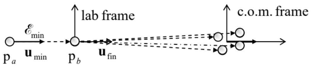
As an example, let us calculate the minimum energy \(\ \mathscr{E}_{\mathrm{min}}\) of a proton \(\ \left(\mathrm{p}_{a}\right)\), necessary for the well-known high-energy reaction that generates a new proton-antiproton pair, \(\ \mathrm{p}_{a}+\mathrm{p}_{b} \rightarrow \mathrm{p}+\mathrm{p}+\mathrm{p}+\overline{\mathrm{p}}\), provided that before the collision, the proton \(\ \mathrm{p}_{b}\) had been at rest in the lab frame. This minimum corresponds to the vanishing relative velocity of the reaction products, i.e. their motion with virtually the same velocity \(\ \left(\mathbf{u}_{\mathrm{fin}}\right)\), as seen from the lab frame – see Fig. 10.

Fig. 9.10. A high-energy proton reaction at \(\ \mathscr{E} \approx \mathscr{E}_{\min }\) - schematically.

Due to the momentum conservation, this velocity should have the same direction as the initial velocity \(\ \left(\mathbf{u}_{\min }\right)\) of proton \(\ p_{a}\). This is why two scalar equations: for energy conservation,

\[\ \frac{m c^{2}}{\left(1-u_{\min }^{2} / c^{2}\right)^{1 / 2}}+m c^{2}=\frac{4 m c^{2}}{\left(1-u_{\mathrm{fin}}^{2} / c^{2}\right)^{1 / 2}},\tag{9.80a}\]

and for momentum conservation,

\[\ \frac{m u}{\left(1-u_{\min }^{2} / c^{2}\right)^{1 / 2}}+0=\frac{4 m u_{\mathrm{fin}}}{\left(1-u_{\mathrm{fin}}^{2} / c^{2}\right)^{1 / 2}},\tag{9.80b}\]

are sufficient to find both \(\ u_{\min }\) and \(\ u_{\mathrm{fin}}\). After a conceptually simple but technically somewhat tedious solution of this system of two nonlinear equations, we get

\[\ u_{\min }=\frac{4 \sqrt{3}}{7} c, \quad u_{\mathrm{fin}}=\frac{\sqrt{3}}{2} c.\tag{9.81}\]

Finally, we can use Eq. (73) to calculate the required energy; the result is \(\ \mathscr{E}_{\min }=7 m c^{2}\). (Note that at this threshold, only \(\ 2 m c^{2}\) of the kinetic energy \(\ T_{\min }=\mathscr{E}_{\min }-m c^{2}=6 m c^{2}\) of the initial moving particle, go into the “useful” proton-antiproton pair production.) The proton’s rest mass, \(\ m_{\mathrm{p}} \approx 1.67 \times 10^{-27} \mathrm{~kg}\), corresponds to \(\ m_{\mathrm{p}} c^{2} \approx 1.502 \times 10^{-10} \mathrm{~J} \approx 0.938 \mathrm{GeV}\), so that \(\ \mathscr{E}_{\min } \approx 6.57 \mathrm{GeV}\).

The second, more intelligent way to solve the same problem is to use the center-of-mass (c.o.m.) reference frame that, in relativity, is defined as the frame in that the total momentum of the system vanishes.³⁶ In this frame, at \(\ \mathscr{E}=\mathscr{E}_{\min }\), the velocity and momenta of all reaction products are vanishing, while the velocities of protons \(\ \mathrm{p}_{a}\) and \(\ \mathrm{p}_{b}\) before the collision are equal and opposite, with an initially unknown magnitude \(\ u^{\prime}\). Hence the energy conservation law becomes

\[\ \frac{2 m c^{2}}{\left(1-u^{\prime 2} / c^{2}\right)^{1 / 2}}=4 m c^{2},\tag{9.82}\]

readily giving \(\ u^{\prime}=(\sqrt{3} / 2) c\). (This is of course the same result as Eq. (81) gives for \(\ u_{\text {fin }}\).) Now we can use the fact that the velocity of the proton \(\ \mathrm{p}_{a}\) in the c.o.m. frame is \(\ \left(-u^{\prime}\right)\), to find its lab-frame speed, using the velocity transform (25):

\[\ u_{\min }=\frac{2 u^{\prime}}{1+u^{\prime 2} / c^{2}}.\tag{9.83}\]

With the above result for \(\ u^{\prime}\), this relation gives the same result as the first method, \(\ u_{\min }=(4 \sqrt{3} / 7) c\), but in a simpler way.

---

Reference

²³ Such vectors are said to reside in so-called 4D Minkowski spaces – called after Hermann Minkowski who was the first one to recast (in 1907) the special relativity relations in a form in which the spatial coordinates and time (or rather ct) are treated on an equal footing.

²⁴ I have opted against using special indices (e.g., \(\ \boldsymbol{\beta}_{u}, \gamma_{u}\)) to distinguish Eqs. (17) and (61) here and below, in a hope that the suitable velocity (of either a reference frame or a particle) will be always clear from the context.

²⁵ I am sorry for using, just as in Sec. 6.3, the same traditional notation \(\ (\mathbf{p})\) for the particle’s momentum as had been used earlier for the electric dipole moment. However, since the latter notion will be virtually unused in the balance of this course, this may hardly lead to confusion.

²⁶ Indeed, such a derivation uses additional assumptions, however natural (such as the Lorentz-invariance of \(\ \mathscr{S}\)), i.e. it can hardly be considered as a real proof of the final results, so that they require experimental confirmation. Fortunately, such confirmations have been numerous – see below.

²⁷ See, e.g., CM Sec. 10.3.

²⁸ See, e.g., CM Sec. 2.1.

²⁹ See, e.g., CM Eq. (2.19b).

³⁰ See, e.g., CM Sec. 2.3, in particular Eq. (2.31).

³¹ See, e.g., CM Eq. (2.32).

³² Let me hope that the reader understands that all the layman talk about the “mass to energy conversion” is only valid in a very limited sense of the word. While the Einstein relation (73) does allow the conversion of “massive” particles (with \(\ m \neq 0\)) into particles with \(\ m=0\), such as photons, each of the latter particles also has a non-zero relativistic mass \(\ M\), and simultaneously the energy \(\ \mathscr{E}\) related to this \(\ M\) by Eq. (73).

³³ Please note one more simple and useful relation following from Eqs. (70) and (73): \(\ \mathbf{p}=\left(\mathscr{E} / c^{2}\right) \mathbf{u}\).

³⁴ It may be tempting to interpret this relation as the perpendicular-vector-like addition of the rest energy \(\ m c^{2}\) and the “kinetic energy” \(\ pc\), but from the point of view of the total energy conservation (see below), a better definition of the kinetic energy is \(\ T(u) \equiv \mathscr{E}(u)-\mathscr{E}(0)\).

³⁵ It is briefly reviewed in QM Chapter 9.

³⁶ Note that according to this definition, the c.o.m.’s radius-vector is \(\ \mathbf{R}=\Sigma_{k} M_{k} \mathbf{r}_{k} / \Sigma_{k} M_{k} \equiv \Sigma_{k} \gamma_{k} m_{k} \mathbf{r}_{k} / \Sigma_{k} \gamma_{k} m_{k}\), i.e. is generally different from the well-known non-relativistic expression \(\ \mathbf{R}=\Sigma_{k} m_{k} \mathbf{r}_{k} / \Sigma_{k} m_{k}\).