10.5: Density Effects and the Cherenkov Radiation

For condensed matter, the Coulomb loss estimate made in the last section is not quite suitable, because it is based on the upper cutoff $\ b_{\max } \sim \gamma u / \omega_{\min }$. For the example given above, the incoming electron velocity u is close to $\ 5 \times 10^{7} \mathrm{~m} / \mathrm{s}$, and for the typical value $\ \omega_{\min } \sim 10^{16} \mathrm{~s}^{-1}\left(\hbar \omega_{\min } \sim 10 \mathrm{eV}\right)$, this cutoff $\ b_{\max }$ is of the order of $\ \sim 5 \times 10^{-9} \mathrm{~m}=5 \mathrm{~nm}$. Even for air at ambient conditions, this is somewhat larger than the average distance (~ 2 nm) between the molecules, so that at the high end of the impact parameter range, at $\ b \sim b_{\max }$, the Coulomb loss events in adjacent molecules are not quite independent, and the theory needs some corrections. For condensed matter, with much higher particle density $\ n$, most collisions satisfy the following condition:

$$\ n b^{3}>>1,\tag{10.99}$$

and the treatment of Coulomb collisions as a set of independent events is inadequate. However, this condition enables the opposite approach: treating the medium as a continuum. In the time-domain formulation used in the previous sections of this chapter, this would be a very complex problem, because it would require an explicit description of the medium dynamics. Here the frequency-domain approach, based on the Fourier transform in both time and space, helps a lot, provided that the functions $\ \varepsilon(\omega)$ and $\ \mu(\omega)$ are considered known – either calculated or taken from experiment. Let us have a good look at this approach because it gives some interesting (and practically important) results.

In Chapter 6, we have used the macroscopic Maxwell equations to derive Eqs. (6.118), which describe the time evolution of electrodynamic potentials in a linear medium with frequency-independent $\ \varepsilon$ and $\ \mu$. Looking for all functions participating in Eqs. (6.118) in the form of plane-wave expansion⁴²

$$\ f(\mathbf{r}, t)=\int d^{3} k \int d \omega f_{\mathbf{k}, \omega} e^{i(\mathbf{k} \cdot \mathbf{r}-\omega t)},\tag{10.100}$$

and requiring all coefficients at similar exponents to be balanced, we get their Fourier images:⁴³

$$\ \left(k^{2}-\omega^{2} \varepsilon \mu\right) \phi_{\mathbf{k}, \omega}=\frac{\rho_{\mathbf{k}, \omega}}{\varepsilon}, \quad\left(k^{2}-\omega^{2} \varepsilon \mu\right) \mathbf{A}_{\mathbf{k}, \omega}=\mu \mathbf{j}_{\mathbf{k}, \omega}.\tag{10.101}$$

As was discussed in Chapter 7, in such a Fourier form, the macroscopic Maxwell theory remains valid even for the dispersive (but isotropic and linear!) media, so that Eqs. (101) may be generalized as

$$\ \left[k^{2}-\omega^{2} \varepsilon(\omega) \mu(\omega)\right] \phi_{\mathbf{k}, \omega}=\frac{\rho_{\mathbf{k}, \omega}}{\varepsilon(\omega)}, \quad\left[k^{2}-\omega^{2} \varepsilon(\omega) \mu(\omega)\right] \mathbf{A}_{\mathbf{k}, \omega}=\mu(\omega) \mathbf{j}_{\mathbf{k}, \omega},\tag{10.102}$$

The evident advantage of these equations is that their formal solution is elementary:

$$\ \text{Field potentials in a linear medium}\quad\quad\quad\quad \phi_{\mathbf{k}, \omega}=\frac{\rho_{\mathbf{k}, \omega}}{\varepsilon(\omega)\left[k^{2}-\omega^{2} \varepsilon(\omega) \mu(\omega)\right]}, \quad \mathbf{A}_{\mathbf{k}, \omega}=\frac{\mu(\omega) \mathbf{j}_{\mathbf{k}, \omega}}{\left[k^{2}-\omega^{2} \varepsilon(\omega) \mu(\omega)\right]},\tag{10.103}$$

so that the “only” remaining things to do is, first, to calculate the Fourier transforms of the functions $\ \rho(\mathbf{r}, t)$ and $\ \mathbf{j}(\mathbf{r}, t)$, describing stand-alone charges and currents, using the transform reciprocal to Eq. (100), with one factor $\ 1 / 2 \pi$ per each scalar dimension,

$$\ f_{\mathbf{k}, \omega}=\frac{1}{(2 \pi)^{4}} \int d^{3} r \int d t f(\mathbf{r}, t) e^{-i(\mathbf{k} \cdot \mathbf{r}-\omega t)},\tag{10.104}$$

and then to carry out the integration (100) of Eqs. (103).

For our problem of a single charge $\ q$ uniformly moving through a medium with velocity u,

$$\ \rho(\mathbf{r}, t)=q \delta(\mathbf{r}-\mathbf{u} t), \quad \mathbf{j}(\mathbf{r}, t)=q \mathbf{u} \delta(\mathbf{r}-\mathbf{u} t),\tag{10.105}$$

the first task is easy:

$$\ \rho_{\mathbf{k}, \omega}=\frac{q}{(2 \pi)^{4}} \int d^{3} r \int d t q \delta(\mathbf{r}-\mathbf{u} t) e^{-i(\mathbf{k} \cdot \mathbf{r}-\omega t)}=\frac{q}{(2 \pi)^{4}} \int e^{i(\omega t-\mathbf{k} \cdot \mathbf{u} t)} d t=\frac{q}{(2 \pi)^{3}} \delta(\omega-\mathbf{k} \cdot \mathbf{u}).\tag{10.106}$$

Since the expressions (105) for $\ \rho(\mathbf{r}, t)$ and $\ \mathbf{j}(\mathbf{r}, t)$ differ only by a constant factor u, it is clear that the absolutely similar calculation for the current gives

$$\ \mathbf{j}_{\mathbf{k}, \omega}=\frac{q \mathbf{u}}{(2 \pi)^{3}} \delta(\omega-\mathbf{k} \cdot \mathbf{u}).\tag{10.107}$$

Let us summarize what we have got by now, plugging Eqs. (106) and (107) into Eqs. (103):

$$\ \phi_{\mathbf{k}, \omega}=\frac{1}{(2 \pi)^{3}} \frac{q \delta(\omega-\mathbf{k} \cdot \mathbf{u})}{\varepsilon(\omega)\left[k^{2}-\omega^{2} \varepsilon(\omega) \mu(\omega)\right]}, \quad \mathbf{A}_{\mathbf{k}, \omega}=\frac{1}{(2 \pi)^{3}} \frac{\mu(\omega) q \mathbf{u} \delta(\omega-\mathbf{k} \cdot \mathbf{u})}{\left[k^{2}-\omega^{2} \varepsilon(\omega) \mu(\omega)\right]} \equiv \varepsilon(\omega) \mu(\omega) \mathbf{u} \phi_{\mathbf{k}, \omega}.\tag{10.108}$$

Now, at the last calculation step, namely the integration (100), we are starting to pay a heavy price for the easiness of the first steps. This is why let us think well about what exactly do we need from it. First of all, for the calculation of power losses, the electric field is more convenient to use than the potentials, so let us calculate the Fourier images of E and B. Plugging the expansion (100) into the basic relations (6.7), and again requiring the balance of exponent’s coefficients, we get

$$\ \mathbf{E}_{\mathbf{k}, \omega}=-i \mathbf{k} \phi_{k, \omega}+i \omega \mathbf{A}_{\mathbf{k}, \omega}=i[\omega \varepsilon(\omega) \mu(\omega) \mathbf{u}-\mathbf{k}] \phi_{\mathbf{k}, \omega}, \quad \mathbf{B}_{\mathbf{k}, \omega}=i \mathbf{k} \times \mathbf{A}_{\mathbf{k}, \omega}=i \varepsilon(\omega) \mu(\omega) \mathbf{k} \times \mathbf{u} \phi_{\mathbf{k}, \omega},\tag{10.109}$$

so that Eqs. (100) and (108) yield

$$\ \mathbf{E}(\mathbf{r}, t)=\int d^{3} k \int d \omega \mathbf{E}_{\mathbf{k}, \omega} e^{i(\mathbf{k} \cdot \mathbf{r}-\omega t)}=\frac{i q}{(2 \pi)^{3}} \int d^{3} k \int d \omega \frac{[\omega \varepsilon(\omega) \mu(\omega) \mathbf{u}-\mathbf{k}] \delta(\omega-\mathbf{k} \cdot \mathbf{u})}{\varepsilon(\omega)\left[k^{2}-\omega^{2} \varepsilon(\omega) \mu(\omega)\right]} e^{i(\mathbf{k} \cdot \mathbf{r}-\omega t)}.\tag{10.110}$$

This formula may be rewritten as the temporal Fourier integral (51), with the following r-dependent complex amplitude:

$$\ \mathbf{E}_{\omega}(\mathbf{r})=\int \mathbf{E}_{\mathbf{k}, \omega} e^{i \mathbf{k} \cdot \mathbf{r}} d^{3} k=\frac{i q}{(2 \pi)^{3}} \int \frac{[\omega \varepsilon(\omega) \mu(\omega) \mathbf{u}-\mathbf{k}] \delta(\omega-\mathbf{k} \cdot \mathbf{u})}{\varepsilon(\omega)\left[k^{2}-\omega^{2} \varepsilon(\omega) \mu(\omega)\right]} e^{i \mathbf{k} \cdot \mathbf{r}} d^{3} k.\tag{10.111}$$

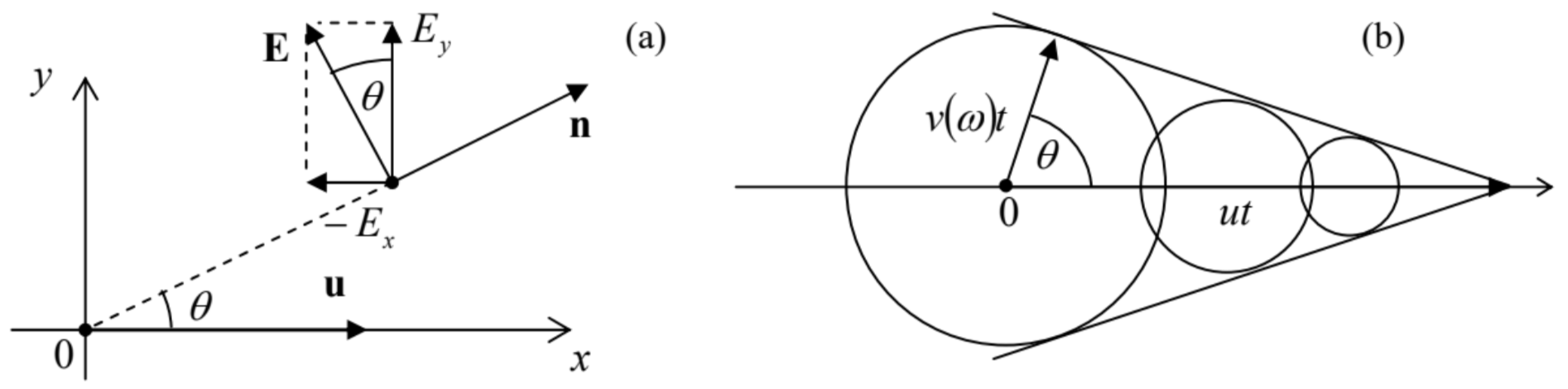
Let us calculate the Cartesian components of this partial Fourier image $\ \mathbf{E}_{\omega}$, at a point separated by distance $\ b$ from the particle’s trajectory. Selecting the coordinates and time origin as shown in Fig. 9.11a, we have $\ \mathbf{r}=\{0, b, 0\}$ and $\ \mathbf{u}=\{u, 0,0\}$, so that only $\ E_{x}$ and $\ E_{y}$ are different from zero. In particular, according to Eq. (111),

$$\ \left(E_{x}\right)_{\omega}=\frac{i q}{(2 \pi)^{3} \varepsilon(\omega)} \int d k_{x} \int d k_{y} \int d k_{z} \frac{\omega \varepsilon(\omega) \mu(\omega) u-k_{x}}{k^{2}-\omega^{2} \varepsilon(\omega) \mu(\omega)} \delta\left(\omega-k_{x} u\right) \exp \left\{i k_{y} b\right\}.\tag{10.112}$$

The delta function kills one integral (over $\ k_{x}$) of the three, and we get

$$\ \left(E_{x}\right)_{\omega}=\frac{i q}{(2 \pi)^{3} \varepsilon(\omega) u}\left[\omega \varepsilon(\omega) \mu(\omega) u-\frac{\omega}{u}\right] \int \exp \left\{i k_{y} b\right\} d k_{y} \int \frac{d k_{z}}{\omega^{2} / u^{2}+k_{y}^{2}+k_{z}^{2}-\omega^{2} \varepsilon(\omega) \mu(\omega)}.\tag{10.113}$$

The internal integral (over $\ k_{z}$) may be readily reduced to the table integral $\ \int d \xi /\left(1+\xi^{2}\right)$, in infinite limits, equal to $\ \pi$,⁴⁴ and result represented as

$$\ \left(E_{x}\right)_{\omega}=-\frac{i \pi q \kappa^{2}}{(2 \pi)^{3} \omega \varepsilon(\omega)} \int \frac{\exp \left\{i k_{y} b\right\}}{\left(k_{y}^{2}+\kappa^{2}\right)^{1 / 2}} d k_{y},\tag{10.114}$$

where the parameter $\ \kappa$ (generally, a complex function of frequency) is defined as⁴⁵

$$\ \kappa^{2}(\omega) \equiv \omega^{2}\left(\frac{1}{u^{2}}-\varepsilon(\omega) \mu(\omega)\right).\tag{10.115}$$

The last integral may be expressed via the modified Bessel function of the second kind:⁴⁶

$$\ \left(E_{x}\right)_{\omega}=-\frac{i q u \kappa^{2}}{(2 \pi)^{2} \omega \varepsilon(\omega)} K_{0}(\kappa b).\tag{10.116}$$

A very similar calculation yields

$$\ \left(E_{y}\right)_{\omega}=\frac{q \kappa}{(2 \pi)^{2} \varepsilon(\omega)} K_{1}(\kappa b).\tag{10.117}$$

Now, instead of rushing to make the final integration (51) over $\ \omega$ to calculate $\ \mathbf{E}(t)$, let us realize that what we need most is the total energy loss through the whole time of the particle’s passage over an elementary distance dx. According to Eq. (4.38), the energy loss per unit volume is

$$\ -\frac{d \mathscr{E}}{d V}=\int \mathbf{j} \cdot \mathbf{E} d t,\tag{10.118}$$

where j is the current of the bound charges in the medium, and should not be confused with the stand-alone incident-particle current (105). This integral may be readily expressed via the partial Fourier image $\ \mathbf{E}_{\omega}$ and the similarly defined image $\ \mathbf{j} \omega$, just as it was done at the derivation of Eq. (54):

$$\ -\frac{d \mathscr{E}}{d V}=\int d t \int d \omega e^{-i \omega t} \int d \omega^{\prime} e^{-i \omega^{\prime} t} \mathbf{j}_{\omega} \cdot \mathbf{E}_{\omega^{\prime}}=2 \pi \int d \omega \int d \omega^{\prime} \mathbf{j}_{\omega} \cdot \mathbf{E}_{\omega^{\prime}} \delta\left(\omega+\omega^{\prime}\right)=2 \pi \int \mathbf{j}_{\omega} \cdot \mathbf{E}_{-\omega} d \omega.\tag{10.119}$$

Let us incorporate the effective Ohmic conductivity $\ \sigma_{\mathrm{ef}}(\omega)$ into the complex permittivity $\ \varepsilon(\omega)$ just as this was discussed in Sec. 7.2, using Eq. (7.46) to write

$$\ \mathbf{j}_{\omega}=\sigma_{\mathrm{ef}}(\omega) \mathbf{E}_{\omega}=-i \omega \varepsilon(\omega) \mathbf{E}_{\omega}.\tag{10.120}$$

As a result, Eq. (119) yields

$$\ -\frac{d \mathscr{E}}{d V}=-2 \pi i \int \varepsilon(\omega) \mathbf{E}_{\omega} \cdot \mathbf{E}_{-\omega} \omega d \omega=4 \pi \operatorname{Im} \int_{0}^{\infty} \varepsilon(\omega)\left|E_{\omega}\right|^{2} \omega d \omega.\tag{10.121}$$

(The last step was possible due to the property $\ \varepsilon(-\omega)=\varepsilon^{*}(\omega)$, which was discussed in Sec. 7.2.)

Finally, just as in the last section, we have to average the energy loss rate over random values of the impact parameter $\ b$:

$$\ -\frac{d \mathscr{E}}{d x}=\int\left(-\frac{d \mathscr{E}}{d V}\right) d^{2} b \approx 2 \pi \int_{b_{\min }}^{\infty}\left(-\frac{d \mathscr{E}}{d V}\right) b d b=8 \pi^{2} \int_{b_{\min }}^{\infty} b d b \int_{0}^{\infty}\left(\left|E_{x}\right|_{\omega}^{2}+\left|E_{y}\right|_{\omega}^{2}\right) \operatorname{Im} \varepsilon(\omega) \omega d \omega.\tag{10.122}$$

Due to the divergence of the functions $\ K_{0}(\xi)$ and $\ K_{1}(\xi)$ at $\ \xi \rightarrow 0$, we have to cut the resulting integral over $\ b$ at some $\ b_{\min }$ where our theory loses legitimacy. (On that limit, we are not doing much better than in the past section). Plugging in the calculated expressions (116) and (117) for the field components, swapping the integrals over $\ \omega$ and $\ b$, and using the recurrence relations (2.142), which are valid for all Bessel functions, we finally get:

$$\ -\frac{d \mathscr{E}}{d x}=\frac{2}{\pi} q^{2} \operatorname{Im} \int_{0}^{\infty}\left(\kappa^{*} b_{\min }\right) K_{1}\left(\kappa^{*} b_{\min }\right) K_{0}\left(\kappa^{*} b_{\min }\right) \frac{d \omega}{\omega \varepsilon(\omega)}.\quad\quad\quad\quad\text{Radiation intensity}\tag{10.123}$$

This general result is valid for a linear medium with arbitrary dispersion relations $\ \varepsilon(\omega)$ and $\ \mu(\omega)$. (The last function participates in Eq. (123) only via Eq. (115) that defines the parameter $\ \kappa$.) To get more concrete results, some particular model of the medium should be used. Let us explore the Lorentz- oscillator model that was discussed in Sec. 7.2, in its form (7.33) suitable for the transition to the quantum-mechanical description of atoms:

$$\ \varepsilon(\omega)=\varepsilon_{0}+\frac{n q^{\prime 2}}{m} \sum_{j} \frac{f_{j}}{\left(\omega_{j}^{2}-\omega^{2}\right)-2 i \omega \delta_{j}}, \quad \text { with } \sum_{j} f_{j}=1 ; \quad \mu(\omega)=\mu_{0}.\tag{10.124}$$

If the damping of the effective atomic oscillators is low, $\ \delta_{j} << \omega_{j}$, as it typically is, and the particle’s speed $\ u$ is much lower than the typical wave’s phase velocity $\ \nu$ (and hence than $\ c$!), then for most frequencies Eq. (115) gives

$$\ \kappa^{2}(\omega) \equiv \omega^{2}\left(\frac{1}{u^{2}}-\frac{1}{\nu^{2}(\omega)}\right) \approx \frac{\omega^{2}}{u^{2}},\tag{10.125}$$

i.e. $\ \kappa \approx \kappa^{*} \approx \omega / u$ is real. In this case, Eq. (123) may be reduced to Eq. (95) with

$$\ b_{\max }=\frac{1.123 u}{\langle\omega\rangle}.\tag{10.126}$$

The good news here is that both approaches (the microscopic analysis of Sec. 4 and the macroscopic analysis of this section) give essentially the same result. The same fact may be also perceived as bad news: the treatment of the medium as a continuum does not give any new results here. The situation somewhat changes at relativistic velocities, at which such treatment provides noticeable corrections (called density effects), in particular reducing the energy loss estimates.

Let me, however, leave these details alone and focus on a much more important effect described by our formulas. Consider the dependence of the electric field components on the impact parameter $\ b$, i.e. on the closest distance between the particle’s trajectory and the field observation point. At $\ b \rightarrow \infty$, we can use, in Eqs. (116)-(117), the asymptotic formula (2.158),

$$\ K_{n}(\xi) \rightarrow\left(\frac{\pi}{2 \xi}\right)^{1 / 2} e^{-\xi}, \text { at } \xi \rightarrow \infty,\tag{10.127}$$

to conclude that if $\ \kappa^{2}>0$, i.e. if $\ \kappa$ is real, the complex amplitudes $\ E_{\omega}$ of both components $\ E_{x}$ and $\ E_{y}$ of the electric field decrease with $\ b$ exponentially. However, let us consider what happens at frequencies where $\ \kappa^{2}(\omega)<0$,⁴⁷ i.e.

$$\ \varepsilon(\omega) \mu(\omega) \equiv \frac{1}{\nu^{2}(\omega)}<\frac{1}{u^{2}}<\frac{1}{c^{2}} \equiv \varepsilon_{0} \mu_{0}.\tag{10.128}$$

(This condition means that the particle’s velocity is larger than the phase velocity of the waves, at this particular frequency.) In these intervals, the parameter $\ \kappa(\omega)$ is purely imaginary, so that the functions $\ \exp \{\kappa b\}$ in the asymptotes (127) of Eqs. (116)-(117) become just phase factors, and the field component amplitudes fall very slowly:

$$\ \left|E_{x}(\omega)\right| \propto\left|E_{y}(\omega)\right| \propto \frac{1}{b^{1 / 2}}.\tag{10.129}$$

This means that the Poynting vector drops as $\ 1/b$, so that its flux through a surface of a round cylinder of radius $\ b$, with the axis on the particle trajectory (i.e. the power flow from the particle), does not depend on b at all. This is an electromagnetic wave emission – the famous Cherenkov radiation.⁴⁸

The direction n of its propagation may be readily found taking into account that at large distances from the particle’s trajectory, the emitted wave has to be locally planar and transverse $\ (\mathbf{n} \perp \mathbf{E})$, so that the so-called Cherenkov angle $\ \theta$ between the vector n and the particle’s velocity u may be simply found from the ratio of the electric field components – see Fig. 14a:

$$\ \tan \theta=-\frac{E_{x}}{E_{y}}.\tag{10.130}$$

Fig. 10.14. (a) The Cherenkov radiation’s propagation angle $\ \theta$, and (b) its interpretation.

The ratio on the right-hand side may be calculated by plugging the asymptotic formula (127) into Eqs. (116) and (117) and calculating their ratio:

$$\ \tan \theta=-\frac{E_{x}}{E_{y}}=\frac{i \kappa u}{\omega}=\left[\varepsilon(\omega) \mu(\omega) u^{2}-1\right]^{1 / 2}=\left(\frac{u^{2}}{\nu^{2}(\omega)}-1\right)^{1 / 2},\tag{10.131a}$$

so that

$$\ \cos \theta=\frac{\nu(\omega)}{u}<1.\quad\quad\quad\quad\text{Cherenkov angle}\tag{10.131b}$$

Remarkably, this direction does not depend on the emission time $\ t_{\mathrm{ret}}$, so that the radiation of frequency $\ \omega$, at each instant, forms a hollow cone led by the particle. This simple result allows an evident interpretation (Fig. 14b): the cone’s interior is just the set of all observation points that have already been reached by the radiation, propagating with the speed $\ \nu(\omega)<u$, emitted from all previous points of the particle’s trajectory by the given time $\ t$. This phenomenon is closely related to the so-called Mach cone in fluid dynamics,⁴⁹ besides that in the Cherenkov radiation, there is a separate cone for each frequency (of the range in which $\ \nu(\omega)<u)$: the smaller is the $\ \varepsilon(\omega) \mu(\omega)$ product, i.e. the higher is the wave velocity $\ \nu(\omega)=1 /[\varepsilon(\omega) \mu(\omega)]^{1 / 2}$, the broader is the cone, so that the earlier the corresponding “shock wave” arrives to an observer. Please note that the Cherenkov radiation is a unique radiative phenomenon: it takes place even if a particle moves without acceleration, and (in agreement with our analysis in Sec. 2), is impossible in free space, where $\ \nu(\omega)=c=\mathrm{const}$ is larger than $\ u$ for any particle.

The Cherenkov radiation’s intensity may be also readily found by plugging the asymptotic expression (127), with imaginary $\ \kappa$, into Eq. (123). The result is

$$\ -\frac{d \mathscr{E}}{d x} \approx\left(\frac{\mathscr{F} e}{4 \pi}\right)^{2} \int_{\nu(\omega)<u} \omega\left(1-\frac{\nu^{2}(\omega)}{u^{2}}\right) d \omega.\quad\quad\quad\quad\text{Cherenkov radiation: intensity}\tag{10.132}$$

For non-relativistic particles $\ (u<<c)$, the Cherenkov radiation condition $\ u>\nu(\omega)$ may be fulfilled only in relatively narrow frequency intervals where the product $\ \varepsilon(\omega) \mu(\omega)$ is very large (usually, due to optical resonance peaks of the electric permittivity – see Fig. 7.5 and its discussion). In this case, the emitted light consists of a few nearly-monochromatic components. On the contrary, if the condition $\ u>\nu(\omega)$, i.e. $\ u^{2} / \varepsilon(\omega) \mu(\omega)>1$ is fulfilled in a broad frequency range (as it is for ultra-relativistic particles in condensed media), the radiated power, according to Eq. (132), is dominated by higher frequencies of the range – hence the famous bluish color of the Cherenkov radiation glow from water-filled nuclear reactors– see Fig. 15.

The Cherenkov radiation is broadly used for the detection of radiation in high energy experiments for particle identification and speed measurement (since it is easy to pass the particles through layers of various density and hence of various dielectric constant values) – for example, in the so-called Ring Imaging Cherenkov (RICH) detectors that have been designed for the DELPHI experiment⁵⁰ at the Large Electron-Positron Collider (LEP) in CERN.

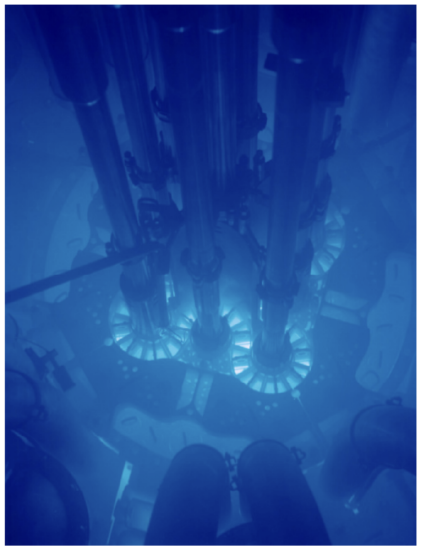Fig. 10.15. The Cherenkov radiation glow from the Advanced Test Reactor of the Idaho National Laboratory in Arco, ID. (Adapted from http://en.Wikipedia.org/wiki/Cherenkov_radiation under the Creative Commons CC-BY-SA-2.0 license.)

A little bit counter-intuitively, the formalism described in this section is also very useful for the description of an apparently rather different effect – the so-called transition radiation that takes place when a charged particle crosses a border between two media.⁵¹ The effect may be interpreted as the result of the time dependence of the electric dipole formed by the moving charge q and its mirror image $\ q^{\prime}$ in the counterpart medium – see Fig. 16.

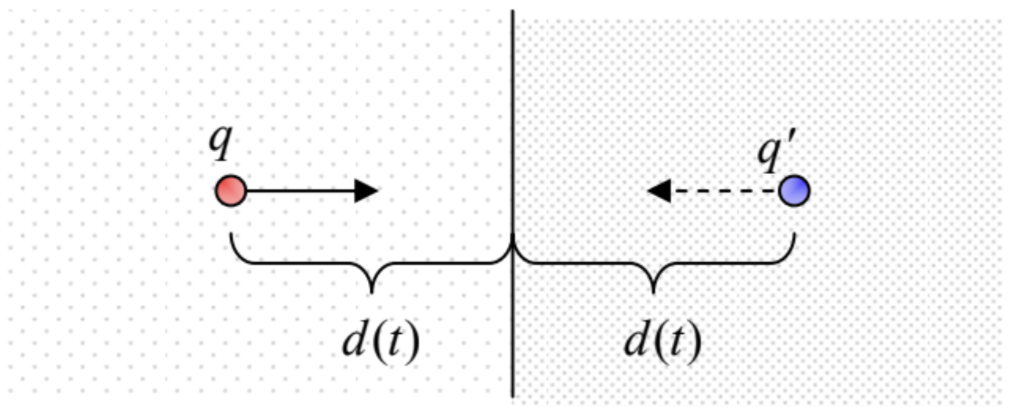Fig. 10.16. The transition radiation’s physics.

In the non-relativistic limit, this effect allows a straightforward description combining the electrostatics picture of Sec. 3.4 (see Fig. 3.9 and its discussion), and Eq. (8.27), corrected for the media polarization effects. However, if the particle’s velocity $\ u$ is comparable with the phase velocity of waves in either medium, the adequate theory of the transition radiation becomes very close to that of the Cherenkov radiation.

In comparison with the Cherenkov radiation, the transition radiation is rather weak, and its practical use (mostly for the measurement of the relativistic factor $\ \gamma$, to which the radiation intensity is nearly proportional) requires multi-layered stacks.⁵² In these systems, the radiation emitted at sequential borders may be coherent, and the system’s physics may become close to that of the free-electron lasers mentioned in Sec. 4.

---

Reference

⁴² All integrals here and below are in infinite limits, unless specified otherwise.

⁴³ As was discussed in Sec. 7.2, the Ohmic conductivity of the medium (generally, also a function of frequency) may be readily incorporated into the dielectric permittivity: $\ \varepsilon(\omega) \rightarrow \varepsilon_{\mathrm{ef}}(\omega)+i \sigma(\omega) / \omega$. In this section, I will assume that such incorporation, which is especially natural for high frequencies, has been performed, so that the current density $\ \mathbf{j}(\mathbf{r}, t)$ describes only stand-alone currents – for example, the current (105) of the incident particle.

⁴⁴ See, e.g., MA Eq. (6.5a).

⁴⁵ The frequency-dependent parameter $\ \kappa(\omega)$ should not be confused with the dc low-frequency dielectric constant $\ \kappa \equiv \varepsilon(0) / \varepsilon_{0}$, which was discussed in Chapter 3.

⁴⁶ As a reminder, the main properties of these functions are listed in Sec. 2.7 – see, in particular, Fig. 2.22 and Eqs. (2.157)-(2.158).

⁴⁷ Strictly speaking, the inequality $\ \kappa^{2}(\omega)<0$, does not make sense for a medium with a complex product $\ \varepsilon(\omega) \mu(\omega)$, and hence complex $\ \kappa^{2}(\omega)$. However, in a typical medium where particles can propagate over substantial distances, the imaginary part of the product $\ \varepsilon(\omega) \mu(\omega)$ does not vanish only in very limited frequency intervals, much more narrow than the intervals that we are discussing now – please have one more look at Fig. 7.5.

⁴⁸ This radiation was observed experimentally by Pavel Alekseevich Cherenkov (in older Western texts, “Čerenkov”) in 1934, with the observations explained by Ilya Mikhailovich Frank and Igor Yevgenyevich Tamm in 1937. Note, however, that the effect had been predicted theoretically as early as in 1889 by the same Oliver Heaviside whose name was mentioned in this course so many times – and whose genius I believe is still underappreciated.

⁴⁹ Its brief discussion may be found in CM Sec. 8.6.

⁵⁰ See, e.g., http://delphiwww.cern.ch/offline/phy...-detector.html. For a broader view at radiation detectors (including the Cherenkov ones), the reader may be referred, for example, to the classical text by G. F. Knoll, Radiation Detection and Measurement, 4^th ed., Wiley, 2010, and a newer treatment by K. Kleinknecht, Detectors for Particle Radiation, Cambridge U. Press, 1999.

⁵¹ The effect was predicted theoretically in 1946 by V. Ginzburg and I. Frank, and only later observed experimentally.

⁵² See, e.g., Sec. 5.3 in K. Kleinknecht’s monograph cited above.