
8.1: Interaction of Radiation with Matter


- Last updated
- Mar 4, 2022
- Save as PDF

( \newcommand{\kernel}{\mathrm{null}\,}\)
Cross Section
Classically, the cross section is the area on which a colliding projectile can impact. Thus for example the cross section of a spherical target of radius r is just given by πr2. The cross section has then units of an area. Let’s consider for example a nucleus with mass number A. The radius of the nucleus is then R≈R0A1/3=1.25A1/3fm and the classical cross section would be σ=πR20A2/3≈5A2/3fm2. For a typical heavy nucleus, such as gold, A = 197, we have σ≈100fm2=1 barn ( symbol b,1b=10−28 m2=10−24 cm2=100fm2.
When scattering a particle off a target however, what becomes important is not the head-on collision (as between balls) but the interaction between the particle and the target (e.g. Coulomb, nuclear interaction, weak interaction etc.). For macroscopic objects the details of these interactions are lumped together and hidden. For single particles this is not the case, and for example we can as well have a collision even if the distance between projectile and target is larger than the target radius. Thus the cross section takes on a different meaning and it is now defined as the effective area or more precisely as a measure of the probability of a collision. Even in the classical analogy, it is easy to see why the cross section has this statistical meaning, since in a collision there is a certain (probabilistic) distribution of the impact distance. The cross section also describes the probability of a given (nuclear) reaction to occur, a reaction that can be generally written as:
a+X→X′+b or X(a,b)X′
where X is an heavy target and a a small projectile (such as a neutron, proton, alpha...) while X′ and b are the reaction products (again with b being nucleons or light nucleus, or in some cases a gamma ray).
Then let Ia be the current of incoming particles, hitting on an heavy (hence stationary) target. The heavy product X′ will also be almost stationary and only b will escape the material and be measured. Thus we will observe the b products arriving at a detector at a rate Rb. If there are n target nuclei per unit area, the cross section can then be written as
σ=RbIan
This quantity do not always agree with the estimated cross section based on the nucleus radius. For example, proton scattering x-section can be higher than neutrons, because of the Coulomb interaction. Neutrinos x-section then will be even smaller, because they only interact via the weak interaction.
Differential Cross Section
The outgoing particles (b) are scattered in all directions. However most of the time the detector only occupies a small region of space. Thus we can only measure the rate Rb at a particular location, identified by the angles ϑ,φ. What we are actually measuring is the rate of scattered particles in the small solid angle dΩ,r(ϑ,φ), and the relevant cross section is the differential cross section
dσdΩ=r(ϑ,φ)4πIan
From this quantity, the total cross section, defined above, can be calculated as
σ=∫4πdσdΩdΩ=∫π0sinϑdϑ∫2π0dφdσdΩ
(Notice that having added the factor 4π gives σ=4πdσdΩ for constant dσdΩ).
Doubly differential cross section
When one is also interested in the energy of the outgoing particles Eb, because this can give information e.g. on the structure of the target or on the characteristic of the projectile-target interaction, the quantity that is measured is the cross section as a function of energy. This can be simply
dσdEb
if the detector is energy-sensitive but collect particles in any direction, or the doubly differential cross section
d2σdΩdEb
Neutron Scattering and Absorption
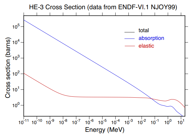
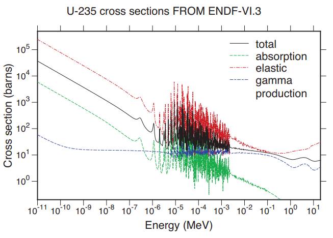
When neutrons travel inside a material, they will undergo scattering (elastic and inelastic) as well as other reactions, while interacting with the nuclei via the strong, nuclear force. Given a beam of neutron with intensity I0, when traveling through matter it will interact with the nuclei with a probability given by the total cross section σT. At high energies, reactions such as (n,p), (n,α) are possible, but at lower energy usually what happens is the capture of the neutron (n,γ) with the emission of energy in the form of gamma rays. Then, when crossing a small region of space dx the beam is reduced by an amount proportional to the number of nuclei in that region:
dI=−I0σTndx→I(x)=I0e−σTnx
This formula, however, is too simplistic: on one side the cross section depends on the neutron energy (the cross section increases at lower velocity as 1/v and at higher energies, the cross section can present some resonances – some peaks) and neutrons will lose part of their energy while traveling, thus the actual cross section will depend on the position. On the other side, not all reactions are absorption reactions, many of them will ”produce” another neutron (i.e., they will only change the energy of the neutron or its direction, thus not attenuating the beam). We then need a better description of the fate of a neutron beam in matter. For example, when one neutron with energy ∼1MeV enters the material, it is first slowed down by elastic and inelastic collisions and it is then finally absorbed.
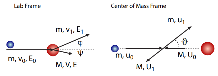
We then want to know how many collisions are necessary to slow down a neutron and to calculate that, we first need to know how much energy does the neutron loose in one collision. Different materials can have different cross sections, however the energy exchange in collision is much higher the lightest the target. Consider an elastic collision with a nucleus of mass M. In the lab frame, the nucleus is initially at rest and the neutron has energy E0 and momentum mv0. After the scattering, the neutron energy is E1, speed →v1 at an angle φ with →v0, while the nucleus recoil gives a momentum M→V at an angle ψ (I will use the notation w for the
magnitude of a vector →w,w=|→w|). The collision is better analyzed in the center of mass frame, where the condition of elastic scattering implies that the relative velocities only change their direction but not their magnitude.
The center of mass velocity is defined as →vCM=m→v0+M˙V0m+M=mm+M→v0. Relative velocities in the center of mass frame are defined as →u=→v−→vCM. We can calculate the neutron (kinetic) energy after the collision from E1=12m|→v1|2. An expression for |→v1|2 is obtained from the CM speed:
|→v1|2=|→u1+→vCM|2=|→u1|2+|→vCM|2+2→u1⋅→vCM=u21+v2CM+2u1vCMcosϑ
where we defined ϑ as the scattering angle in the center of mass frame (see Figure 8.1.3).
Given the assumption of elastic scattering, we have |→u1|=|→u0|=u0, but u0=v0−vCM=v0(1−mm+M)=Mm+Mv0.
Finally, we can express everything in terms of v0:
|→v1|2=M2(m+M)2v20+m2(m+M)2v20+2M(m+M)v0m(m+M)v0cosϑ=v20M2+m2+2mMcosϑ(m+M)2
We now simplify this expression by making the approximation M/m≈A, where A is the mass number of the nucleus.
In terms of the neutron energy, we finally have
E1=E0A2+1+2Acosϑ(A+1)2,
This means that the final energy can be equal to E0 (the initial one) if ϑ=0 – corresponding to no collision– and reaches a minimum value of E1=E0(A−1)2(A+1)2=αE0 for ϑ=π (here α=(A−1)2(A+1)2).
Notice that from this expression it is clear that the neutron loose more energy in the impact with lighter nuclei, in particular all the energy in the impact with proton:
- If A≫1,E1≈E0A2+2AcosϑA2≈E0, that is, almost no energy is lost.
- If A=1,E1=E02+2cosϑ4=E0cos(ϑ2)2, and for ϑ=π all the energy is lost.
For low energy, the cross section is independent of ϑ thus we have a flat distribution of the outgoing energies: the probability to scatter in any direction is constant, thus P(cosϑ)=12. What is the probability of a given energy E1?
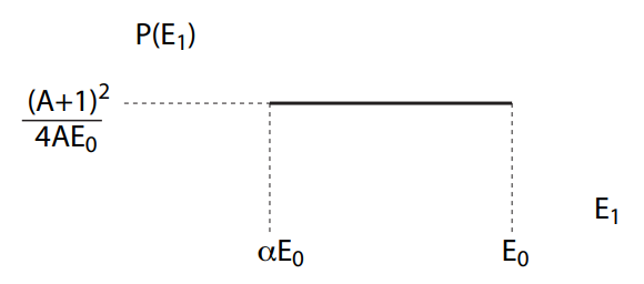
We have P(E1)dE1=−P(cosϑ)d(cosϑ)=−12sinϑdϑ. Then, since dEdϑ=−2E0A(A+1)2sinϑ, the probability of a given scattering energy is constant, as expected, and equal to P(E1)=(A+1)24E0A. Notice that the probability is different than zero only for αE0≤E1≤E0. The average scattering energy is then ⟨E1⟩=E01+α2 and the average energy lost in a scattering event is ⟨Eloss⟩=E01−α2.
It still requires many collision to lose enough energy so that a final capture is probable. How many?
The average energy after one collision is ⟨E1⟩=E01+α2. After two collision it can be approximated by ⟨E2⟩≈ ⟨E1⟩1+α2=E0(1+α2)2. Then, after n collision, we have ⟨En⟩≈E0(1+α2)n=E0(⟨E1⟩E0)n. Thus, if we want to know how many collisions are needed to reach an average thermal energy Eth=⟨En⟩ we need to calculate n:
EthE0=⟨En⟩E0≈(⟨E1⟩E0)n→nlog(⟨E1⟩E0)=log(EthE0)→n=log(EthE0)/log(⟨E1⟩E0)
However, this calculation is not very precise, since the approximation we made, that we can calculate the average energy after the nth scattering ⟨En⟩ considering only the average after the (n−1)th scattering is not a good one, since the energy distribution is not peaked around its average (but is quite flat). Consider instead the quantity log (En−1En) and take the average over the possible final energy (note that this is the same as calculating for the first collision):
⟨log(En−1En)⟩=∫En−1αEn−1log(En−1En)P(En)dEn=∫En−1αEn−1log(En−1En)(A+1)24AEn−1dEn=1+(A−1)22Alog(A−1A+1)
The expression ξ=⟨log(En−1En)⟩ does not depend on the energy, but only on the moderating nucleus (it depends on A).
Then we have that ⟨log(E0En)⟩=⟨log(En−1En)n⟩ or ⟨log(En)⟩=log(E0)−nξ, from which we can calculate the En En number of collisions needed to arrive at a certain energy:
n(E0→Eth)=1ξlog(EthE0)
with ξ the average logarithmic energy loss:
ξ=1+(A−1)22Alog(A−1A+1)
For protons (1H),ξ=1 and it takes 18 collision to moderate neutrons emitted in fission (E=2MeV) while 2200 collisions are needed in 238U.
Material AαξnH10118.2H201&16−0.92019.8D20.1110.72525.1He40.3600.42542.8Be90.6400.20788.1C120.7160.158115U2380.9830.00842172
Charged particle interaction
Charged particles (such as alpha particles and electrons/positrons) going through matter can interact both with the nuclei –via the nuclear interaction and the coulomb interaction– and with the electron cloud –via the Coulomb interaction. Although the effects of a collision with the light electron is going to affect the colliding particle much less than an impact with the heavy nucleus, the probability of such a collision is much higher. This can be intuitively understood by analyzing the effective size of the nucleus and the electronic cloud. While the nucleus have a radius of about 8fm, the atomic radius is on the order of angstroms (or 105fm) Then the area offered to the incoming particle is on the order of π(8fm)2∼200fm2=2 barns .
On the other side, the electronic cloud present an area of π(105fm)2∼π108 barns to the incoming particle. Although the cross section of the reaction (or the probability of interaction between particles) is not the same as the area (as it is for classical particles) still these rough estimates give the correct order of magnitude for it.
Thus the interactions with the electrons in the atom dominate the overall charged particle/matter interaction. However the collision with the nucleus gives rise to a peculiar angular distribution, which is what lead to the discovery of the nucleus itself. We will thus study both types of scattering for light charged projectiles such as alpha particles and protons.
Alpha particles collision with the electronic cloud
Let us consider first the slowing down of alpha particles in matter. We first analyze the collision of one alpha particle with one electron.
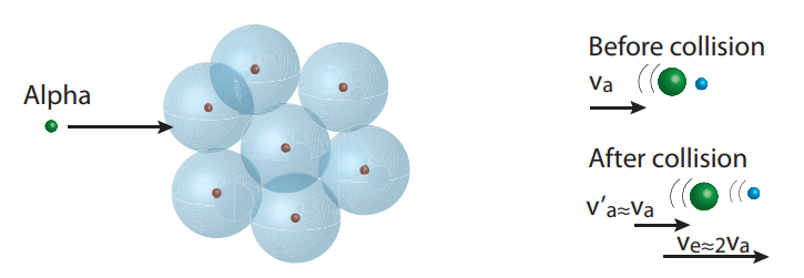
If the collision is elastic, momentum and kinetic energy are conserved (here we consider a classical, non-relativistic collision)
mαvα=mαv′α+meve,mαv2α=mαv′2α+mev2e
Solving for v′a and ve we find:
v′α=vα−2vαmeme+mα,ve=2vαmαme+mα
Since me/mα≪1, we can approximate the electron velocity by ve≈2vα. Then the change in energy for the alpha particle, given by the energy acquired by the electron, is
ΔE=12mev2e=12me(2vα)2=4memαEα
thus the alpha particle looses a tiny fraction of its original energy due to the collision with a single electron:
ΔEαEα∼memα≪1
The small fractional energy loss yields the characteristics of alpha slowing down:
- Thousands of events (collisions) are needed to effectively slow down and stop the alpha particle
- As the alpha particle momentum is barely perturbed by individual collisions, the particle travels in a straight line inside matter.
- The collisions are due to Coulomb interaction, which is an infinite-range interaction. Then, the alpha particle interacts simultaneously with many electrons, yielding a continuous slowing down until the particle is stopped and a certain stopping range.
- [ The electrons which are the collision targets get ionized, thus they lead to a visible trail in the alpha particle path (e.g. in cloud chambers)
We calculated the energy lost by the alpha particle in the collision with one electron. A more important quantity is the average energy loss of the particle per unit path length, which is called the stopping power.
We consider an alpha particle traveling along the x direction and interacting with an electron at the origin of the x-axis and at a distance b from it. It is natural to assume cylindrical coordinates for this problem.
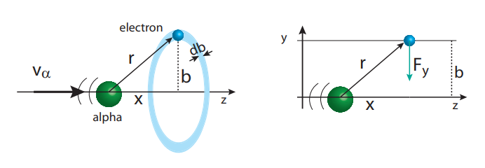
The change in momentum of the electron is given by the Coulomb force, integrated over the interaction time. The Coulomb interaction is given by →F=eQ4πϵ0ˆr|→r|2, where →r=rˆr is the vector joining the alpha to the electron. Only the component of the force in the “radial” (y) direction gives rise to a change in momentum (the longitudinal force when integrated has a zero net contribution), so we calculate →F⋅ˆy=|F|ˆr⋅ˆy. From the figure above we have ˆr⋅ˆy=b(x2+b2)1/2 and finally the force Fy=eQ4πϵ0b(x2+b2)3/2. The change in momentum is then
Δp=∫∞0Fydt=∫∞−∞dxvαe2Zα4πϵ0b(x2+b2)3/2
where we used the relation dxdt=vα between the alpha particle velocity (which is constant with time under our assumptions) and Q=Zαe=2e. By considering the electron initially at rest we have
Δp=pe=e2Z4πϵ0vb∫dξ(1+ξ2)3/2=2e2Zα4πϵ0vαb
where we used ξ=x/b. Then, the energy lost by the alpha particle due to one electron is
ΔE=p2e2m=2e4Z2α(4πϵ0)2mev2b2
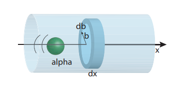
We now sum over all electrons in the material. The number of electrons in an infinitesimal cylinder is dNe=ne2πbdbdx, where ne is the electron’s number density (which can be e.g. calculate from ne=NAZρA, with NA Avogadro’s number and ρ the mass density of the material).
Then
−dE=2πdx∫neΔEbdb→dEdx=−2π∫neΔE(b)bdb=−4πe4Z2αne(4πϵ0)2mev2α∫dbb
The integral should be evaluated between 0 and ∞. However this is not mathematically possible (since it diverges) and it is also physically unsound. We expect in fact to have a distance of closest approach such that the maximum energy exchange (as in the hard-on collision studied previously) is achieved. We had obtained Ee=2mev2α. Then we set this energy equal to the electron’s Coulomb potential energy: Ee≈14πϵ0e2bmin from which we obtain
bmin∼14πϵ0e22mev2α
The maximum b is given by approximately the Bohr radius (or the atom’s radius). This can be calculated by setting 14πϵ0e2bmax∼EI where EI is the mean excitation energy of the atomic electrons. Then what we are stating is that the maximum impact parameter is the one at which the minimum energy exchange happen, and this minimum energy is the minimum energy required to excite (knock off) an electron out of the atom. Although the mean excitation energy of the atomic electrons is a concept related to the ionization energy (which is on the order of 4 − 15eV) here EI is taken as an empirical parameter, which has been found to be well approximated by EI∼10ZeV (with Z the atomic number of the target). Finally we have
bmaxbmin=2mev2αZαEI
and the stopping power is
−dEdx=4πe4Z2αne(4πϵ0)2mev2αln(bmaxbmin)=4πe4Z2αne(4πϵ0)2mev2αlnΛ
with Λ called the Coulomb logarithm.
Since the stopping power, or energy lost per unit length, is given by the energy lost in one collision (or ΔE) times the number of collision (given by the number of electron per unit volume times the probability of one electron collision, given by the cross section) we have the relation:
−dEdx=σcneΔE
from which we can obtain the cross section itself. Since ΔE=2mev2, we have
σc=2πe4Z2α(4πϵ0)2m2ev4αlnΛ
This can also be rewritten in terms of more general constants. We define the classical electron radius as
re=14πϵ0e2mec2∼2.8fm,
which is the distance at which the Coulomb energy is equal to the rest mass. Although this is not close to the real size of an electron (as for example we would expect the electron radius –if it could be well defined– to be much smaller than the nucleus radius) it gives the correct order of magnitude of the effective area in the collision by charged particles. Also we write β=vc, so that
σc=2πr2eZ2αβ4lnΛ
Since β is usually quite small for alpha particles, the cross section can be quite large. For example for a typical alpha energy of Eα=4MeV, and its rest mass mαc2∼4000MeV, we have v2c2∼2×10⁻³. The Coulomb logarithm is on the order of lnΛ∼5−15, while 2πr2e∼12 barn. Then the cross section is σc∼124⋅106/4⋅10b=5×106b.
This is defined by
1/lα=−1EdEdx.
Then we can write an exponential decay for the energy as a function of distance traveled inside a material: E(x)=E0exp(−x/lα). Thus the stopping length also gives the distance at which the energy has been reduced by 1/e(≈63%).
In terms of the cross section the stopping length is:
1/lα=4m2mασcZn,
where n, the atomic number density can be expressed in terms of the mass density and the Avogadro number, n=ρANA.
Stopping length for lead: 1/lα=4×104 cm−1 or lα=2.5×10⁻⁵ cm. The range of the particle in the material is however many stopping lengths (on the order of 10), thus the range in lead is around 2.5μm.
The range is more precisely defined as the distance a particle travels before coming to rest. Then, the range for a particle of initial kinetic energy Eα is defined as
R(Eα)=∫r(E=0)r(Eα)dx=−∫Eα0(dEdx)−1dE
Notice that these is a strong dependence of the stopping power on the mass density of the material (a linear dependence) such that heavier materials are better at stopping charged particles.
However, for alpha particles, it doesn’t take a lot to be stopped. For example, they are stopped in 5 mm of air.
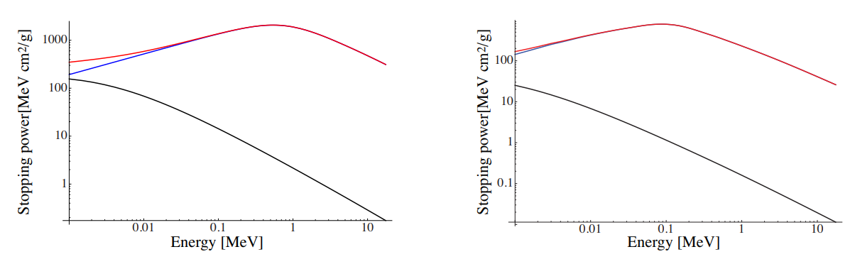
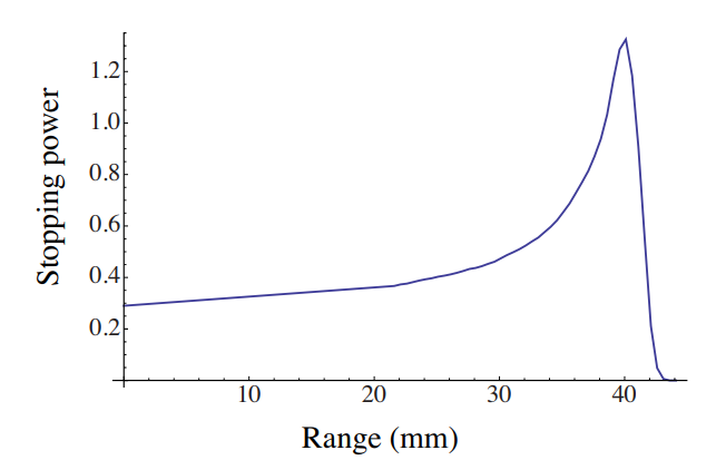
The Bragg curve describes the Stopping power as a function of the distance traveled inside matter. As the stopping power (and the cross section) increase at lower energies, toward the end of the trajectory there is an increase in energy lost per unit length. This gives rise to a characteristic Bragg peak in the curve. This feature is exploited for example for radiation therapy, since it allows a more precise spatial delivery of the dose at the desired location.
B. Rutherford - Coulomb scattering
Elastic Coulomb scattering is called Rutherford scattering because of the experiments carried out in Rutherford lab in 1911-1913 that lead to the discovery of the nucleus. The experiments involved scattering alpha particles off a thin layer of gold and observing the scattering angle (as a function of the gold layer thickness).
The interaction is given as before by the Coulomb interaction, but this time between the alpha and the protons in the nucleus. Thus we have some difference with respect to the previous case. First, the interaction is repulsive (as both particle have positive charges). Then more importantly, the projectile is now the smaller particle, thus loosing considerable energy and momentum in the interaction.
What we want to calculate in this interaction is the differential cross section dσdΩ. The differential (infinitesimal) cross section can be calculated (in a classical picture) by considering the impact parameter b and the small annular region between b and b+db:
dσ=2πbdb
Then the differential cross-section, calculated from the solid angle dΩ=dφsinϑdϑ→2πsinϑdϑ (given the symmetry about φ), is:
dσdΩ=2πbdb2πsinϑdϑ=bsinϑdbdϑ
What we need is then a relationship between the impact parameter and the scattered angle ϑ (see figure).
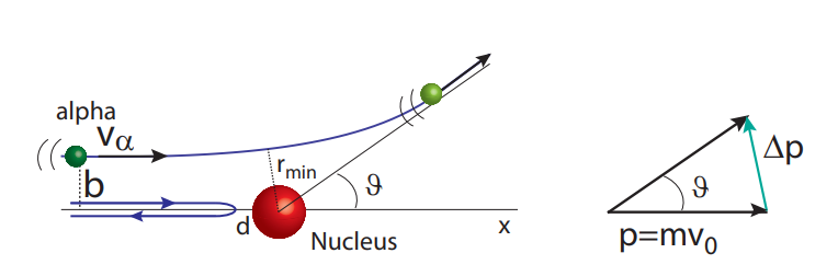
In order to find b(ϑ) we study the variation of energy, momentum and angular momentum. Conservation of energy states that:
12mv20=12mv2+zZe24πϵ0r
which gives the minimum distance (or distance of closest approach) for zero impact parameter b = 0, that happens when the particle stops and gets deflected back: 12mv20=zZe24πϵ0d.
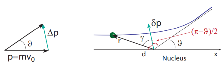
The momentum changes due to the Coulomb force, as seen in the case of interaction with electrons. Here however the nucleus almost does not acquire any momentum at all, so that only the momentum direction is changed, but not its absolute value: initially the momentum is p0=mv0 along the incoming (x) direction, and at the end of the interaction it is still mv0 but along the ϑ direction. Then the change in momentum is Δp=2p0sinϑ2=2mv0sinϑ2 (see Fig. above). This momentum difference is along the direction δˆp, which is at an angle π−ϑ2 with x. We then switch to a reference frame where →r={r,γ}, with r the distance |→r| and γ the angle between the particle position and δˆp.
The momentum change is brought about by the force in that direction:
Δp=∫∞0→F⋅δˆpdt=zZe24πϵ0∫∞0ˆr⋅δˆp|r2|dt=zZe24πϵ0∫∞0cosγr2dt
Notice that at t = 0, γ=−π−ϑ2 (as →r is almost aligned with x) and at t = ∞, γ=π−ϑ2 (Fig). How does γ changes with time?
The angular momentum conservation (which is always satisfied in central potential) provides the answer. At t = 0, the angular momentum is simply L=mv0b. At any later time, we have L=m→r×→v. In the coordinate system →r={r,γ} the velocity has a radial and an angular component:
→v=˙rˆr+r˙γ→γ
and only this last one contributes to the angular momentum (the other being parallel):
L=mr2dγdt→1r2=˙γv0b
Inserting into the integral we have :
Δp=zZe24πϵ0∫∞0cosγ˙γv0bdt=zZe24πϵ0∫π+ϑ2π−ϑ2cosγv0bdγ=zZe24πϵ0v0b2cosϑ2
By equating the two expressions for Δp, we have the desired relationship between b and ϑ:
2mv0sinϑ2=zZe24πϵ0v0b2cosϑ2→b=zZe24πϵ0mv20cotϑ2
Finally the cross section is:
dσdΩ=(zZe24πϵ0)2(4Ta)−2sin−4(ϑ2)
(where Ta=12mv0 is the incident –alpha– particle kinetic energy). In particular, the Z2, T−2 and sin−4 dependence are in excellent agreement with the experiments. The last dependence is characteristic of single scattering events and observing particles at large angles (although less probable) confirm the presence of a massive nucleus. Consider gold foil of thickness ζ=2μm and an incident beam of 8MeV alpha particles. The impact parameter that gives a scattering angle of 90 degrees or more is b≤d2=14fm. Then the fraction of particles with that impact parameter is ∝πb2, thus we have ζnπb2≈7.5×10⁻⁵ particles scattering at an angle ≥90∘ (with n the target density). Although this is a small number, it is quite large compared to the scattering from a uniformly dense target.
C. Electron stopping in matter
Electrons interact with matter mainly due to the Coulomb interaction. However, there are differences in the interaction effects with respect to heavier particles. The differences between the alpha particle and electron behavior in matter is due to their very different mass:
- Electron-electron collisions change the momentum of the incoming electron, thus deflecting it. Then the path of the electron is not straight anymore.
- The stopping power is much less, so that e.g. the range is 1cm in lead. (remember that the ratio of the energy lost to the initial energy for alpha particles was small, since it was proportional to the ratio of masses -electron to alpha. Here the masses ratio is 1, and we expect a large change in energy).
- Electrons have more often a relativistic speed. For example, electrons emitted in the beta decay travel at relativistic speed.
- There is a second mechanism for deceleration. Since the electrons can undergo rapid changes of velocity due to the collision, it is constantly accelerating (or decelerating) and thus it radiates. This radiation is called Bremsstrahlung, or braking radiation (in German).
The stopping power due to the Coulomb interaction can be calculated in a very similar way to what done for the alpha particle. We obtain:
−dEdx=4π(e24πϵ0)2ZρNAA1mec2β2lnΛ′
Here Λ′ is now a different ratio than the one obtained for the alpha particles, but with a similar meaning: Λ′=√T2mev2(T+mc2)EI, where again we can recognize the ratio of the electron energy (determining the minimum distance) and the mean excitation energy EI (which sets the maximum distance) as well as a correction due to relativistic effects.
A quantum mechanical calculation gives some corrections (for the alpha as well) that become important at relativistic energies (see Krane):
−dEdx=4π(e24πϵ0)2ZρNAA1mec2β2[lnΛ′+ relativistic corrections ]
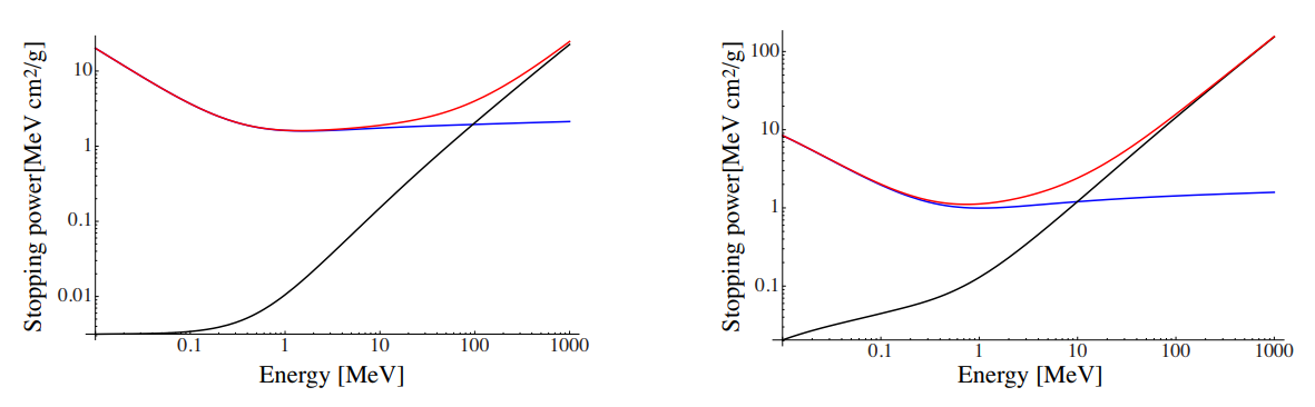
To this stopping power, we must add the effects due to the “braking radiation”. Instead of calculating the exact contribution (see Krane), we just want to estimate the relative contribution of Bremsstrahlung to the Compton scattering. The ratio between the radiation stopping power and the coulomb stopping power is given by
−dEdx|r/−dEdx|c=e2ℏcZfcT+mec2mec2≈T+mec2mec2Z1600
where fc∼10−12 is a factor that takes into account relativistic corrections and remember e2ℏc≈1137. Then the radiation stopping power is important only if T≫mec2 and for large Z. This expression is valid only for relativistic energies; below 1MeV the radiation losses are negligible. Then the total stopping power is given by the sum of the two contributions:
dEdx=dEdx|c+dEdx|r
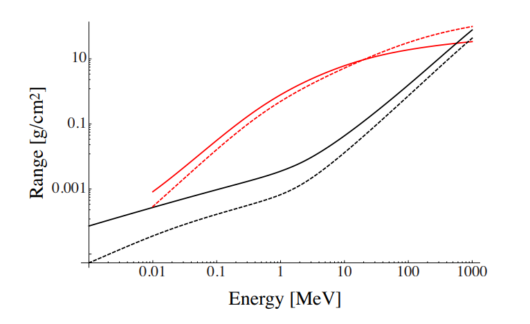
Since the electron do not have a linear path in the materials (but a random path with many collisions) it becomes more difficult to calculate ranges from first principles (in practice, we cannot just take dt=dx/v as done in the calculations for alphas). The ranges are then calculated empirically from experiments in which the energy of monoenergetic electron beams is varied to calculate R(E). NIST provides databases of stopping power and ranges for electrons (as well as for alpha particles and protons, see the STAR database at http://www.nist.gov/pml/data/star/index.cfm. Since the variation with the material characteristics (once normalized by the density) is not large, the range measured for one material can be used to estimate ranges for other materials.
8.1.4 Electromagnetic radiation
The interaction of the electromagnetic radiation with matter depends on the energy (thus frequency) of the e.m. radiation itself. We studied the origin of the gamma radiation, since it derives from nuclear reactions. However, it is interesting to also study the behavior of less energetic radiations in matter.
In order of increasing photon energy, the interaction of matter with e.m. radiation can be classified as:
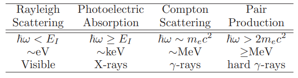
Here EI is the ionization energy for the given target atom.
A classical picture is enough to give some scaling for the scattering cross section. We consider the effects of the interaction of the e.m. wave with an oscillating dipole (as created by an atomic electron).
The electron can be seen as being attached to the atom by a ”spring”, and oscillating around its rest position with frequency ω0. When the e.m. is incident on the electron, it exerts an additional force. The force acting on the electron is F=−eE(t), with E(t)=E0sin(ωt) the oscillating electric field. This oscillating driving force is in addition to the attraction of the electron to the atom ∼−kxe, where k (given by the Coulomb interaction strength and related to the binding energy EI) is linked to the electron’s oscillating frequency by ω20=k/me. The equation of motion for the electron is then
me¨xe=−kxe−eE(t)→¨xe+ω20xe=−emeE(t)
We seek a solution of the form xe(t)=Asin(ωt), then we have the equation
(−ω2+ω20)A=−emeE0→A=1ω2−ω20emeE0
We have already seen that an accelerated charge (or an oscillating dipole) radiates, with a power
P=23e2c3a2
where the accelaration a is here a=−ω2Asin(ωt), giving a mean square acceleration
⟨a2⟩=(ω2ω20−ω2emeE0)212
The radiated power is then
P=13(e2mec2)2ω4(ω20−ω2)2cE20
The radiation intensity is given by I0=cE208π (recall that the e.m. energy density is given by u=12E2 and the intensity, or power per unit area, is then I∼cu). Then we can express the radiated power as cross-section×radiation intensity:
P=σI0
This yields the cross section for the interaction of e.m. radiation with atoms :
σ=8π3(e2mec2)2(ω2ω20−ω2)2
or in SI units:
σ=8π3(e24πϵ0mec2)2(ω2ω20−ω2)2=4πr2e23(ω2ω20−ω2)2
where we used the classical electron radius re.
A. Rayleigh Scattering
We first consider the limit in which the e.m. radiation has very low energy: ω≪ω0. In this limit the electron is initially bound to the atom and the e.m. is not going to change that (and break the bound). We can simplify the frequency factor in the scattering cross-section by ω2ω20−ω2≈ω2ω20, then we have:
σR=8π3(e24πϵ0mec2)2ω4ω40
The Rayleigh scattering has a very strong dependence on the wavelength of the e.m. wave. This is what gives the blue color to the sky (and the red color to the sunsets).
B. Thomson Scattering
Thomson scattering is scattering of e.m. radiation that is energetic enough that the electron appears to be initially unbound from the atom (or a free electron) but not energetic enough to impart a relativistic speed to the electron. (If the electron is a free electron, the final frequency of the electron will be the e.m. frequency).
We are then considering the limit:
ℏω0≪ℏω≪mec2
where the first inequalities tells us that the binding energy is much smaller than the e.m. energy (hence free electron) while the second tells us that the electron will not gain enough energy to become relativistic.
Then we can simplify the factor ω2ω20−ω2=1(ω0/ω)2−1≈−1 and the cross section is simply
σT=8π3(e24πϵ0mec2)2
with σT∼23 barn. Notice that contrasting with the Rayleigh scattering, Thomson scattering cross-section is completely independent of the frequency of the incident e.m. radiation (as long as this is in the given range). Both these two types of scattering are elastic scattering, meaning that the atom is left in the same state as it was initially (so conservation of energy is satisfied without any additional energy coming from the internal atomic energy). Even in Thomson scattering we neglect the recoil of the electron (as stated by the inequality ℏω≪mec2). This means that the electron is not changed by this scattering event (the atom is not ionized) even if in its interaction with the e.m. field it behaves as a free electron.
Notice that the cross section is proportional to the classical electron radius square: σT=8π3r2e.
C. Photoelectric Effect
At resonance ω≈ω0 the cross-section becomes (mathematically) infinite. The resonance condition means that the e.m. energy is equal to the ionization energy EI of the electron. Thus, what it really happens is that the electron gets ejected from the atom. Then our simple model, from which we calculated the cross section, is no longer valid (hence the infinite cross section) and we need QM to fully calculate the cross-section. This is the photoelectric effect. Its cross section is strongly dependent on the atomic number (as σpe∝Z5).
D. Compton Scattering
Compton scattering is the scattering of highly energetic photons from electrons in atoms. In the process the electron acquire an energy high enough to become relativistic and escape the atom (that gets ionized). Thus the scattering is now inelastic (compared to the previous two scattering) and the scattering is an effective way for e.m. radiation to lose energy in matter. At lower energies, we would have the photoelectric effect, in which the photon is absorbed by the atom. The effect is important because it demonstrates that light cannot be explained purely as a wave phenomenon.
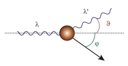
From conservation of energy and momentum, we can calculate the energy of the scattered photon.
Eγ+Ee=E′γ+E′e→ℏω+mec2=ℏω′+√|p|2c2+m2c4
ℏ→k=ℏ→k′+→p→{ℏk=ℏk′cosϑ+pcosφℏk′sinϑ=psinφ
From these equations we find p2=(ω′−ω)c2[ℏ(ω′−ω)−2mc2] and cosφ=√1−ℏ2k′2sin2ϑ/p2. Solving for the change in the wavelength λ=2πk we find (with ω = kc):
\boxed{\Delta \lambda=\frac{2 \pi \hbar}{m_{e} c}(1-\cos \vartheta)} \nonumber
or for the frequency:
\hbar \omega^{\prime}=\hbar \omega\left[1+\frac{\hbar \omega}{m_{e} c^{2}}(1-\cos \vartheta)\right]^{-1} \nonumber
The cross section needs to be calculated from a full QM theory. The result is that
\boxed{\sigma_{C} \approx \sigma_{T} \frac{m_{e} c^{2}}{\hbar \omega}} \nonumber
thus Compton scattering decreases at larger energies.
E. Pair Production
Pair production is the creation of an electron and a positron pair when a high-energy photon interacts in the vicinity of a nucleus. In order not to violate the conservation of momentum, the momentum of the initial photon must be absorbed by something. Thus, pair production cannot occur in empty space out of a single photon; the nucleus (or another photon) is needed to conserve both momentum and energy .
Photon-nucleus pair production can only occur if the photons have an energy exceeding twice the rest mass (m_{e} c^{2}) of an electron (1.022 MeV):
\hbar \omega=T_{e^{-}}+m_{e^{-}} c^{2}+T_{e^{+}}+m_{e^{+}} c^{2} \geq 2 m_{e} c^{2}=1.022 M e V \nonumber
Pair production becomes important after the Compton scattering falls off (since its cross-section is \propto 1 / \omega\)).