2.2: Free Particle- Wave Packets

Let us start our discussion of particular problems with the free 1D motion, i.e. with $U(x, t)=0$. From Eq. (1.29), it is evident that in the 1D case, a similar "fundamental" (i.e. a particular but the most important) solution of the Schrödinger equation (1) is a sinusoidal ("monochromatic") wave $$\Psi_{0}(x, t)=\text { const } \times \exp \left\{i\left(k_{0} x-\omega_{0} t\right)\right\} .$$ According to Eqs. (1.32), it describes a particle with definite momentum $^{2} p_{0}=\hbar k_{0}$ and energy $E_{0}=\hbar \omega_{0}$ $=\hbar^{2} k_{0}^{2} / 2 m$. However, for this wavefunction, the product $\Psi^{*} \Psi$ does not depend on either $x$ or $t$, so that the particle is completely delocalized, i.e. the probability to find it the same along all axis $x$, at all times.

In order to describe a space-localized state, let us form, at the initial moment of time $(t=0)$, a wave packet of the type shown in Fig. 1.6, by multiplying the sinusoidal waveform (15) by some smooth envelope function $A(x)$. As the most important particular example, consider the Gaussian wave packet $$\Psi(x, 0)=A(x) e^{i k_{0} x}, \quad \text { with } A(x)=\frac{1}{(2 \pi)^{1 / 4}(\delta x)^{1 / 2}} \exp \left\{-\frac{x^{2}}{(2 \delta x)^{2}}\right\}$$ (By the way, Fig. 1.6a shows exactly such a packet.) The pre-exponential factor in this envelope function has been selected in the way to have the initial probability density, $$w(x, 0) \equiv \Psi^{*}(x, 0) \Psi(x, 0)=A^{*}(x) A(x)=\frac{1}{(2 \pi)^{1 / 2} \delta x} \exp \left\{-\frac{x^{2}}{2(\delta x)^{2}}\right\}$$ normalized as in Eq. (3), for any parameters $\delta x$ and $k_{0} \cdot{ }^{3}$

To explore the evolution of this wave packet in time, we could try to solve Eq. (1) with the initial condition (16) directly, but in the spirit of the discussion in Sec. 1.5, it is easier to proceed differently. Let us first represent the initial wavefunction (16) as a sum (1.67) of the eigenfunctions $\psi_{k}(x)$ of the corresponding stationary 1D Schrödinger equation (1.60), in our current case $$-\frac{\hbar^{2}}{2 m} \frac{d^{2} \psi_{k}}{d x^{2}}=E_{k} \psi_{k}, \quad \text { with } E_{k} \equiv \frac{\hbar^{2} k^{2}}{2 m},$$ which are simply monochromatic waves, $$\psi_{k}=a_{k} e^{i k x} .$$ Since (as was discussed in Sec. 1.7) at the unconstrained motion the spectrum of possible wave numbers $k$ is continuous, the sum (1.67) should be replaced with an integral: 4 $$\Psi(x, 0)=\int a_{k} e^{i k x} d k$$ Now let us notice that from the point of view of mathematics, Eq. (20) is just the usual Fourier transform from the variable $k$ to the "conjugate" variable $x$, and we can use the well-known formula of the reciprocal Fourier transform to write $$a_{k}=\frac{1}{2 \pi} \int \Psi(x, 0) e^{-i k x} d x=\frac{1}{2 \pi} \frac{1}{(2 \pi)^{1 / 4}(\delta x)^{1 / 2}} \int \exp \left\{-\frac{x^{2}}{(2 \delta x)^{2}}-i \widetilde{k} x\right\} d x, \quad \text { where } \widetilde{k} \equiv k-k_{0} .$$ This Gaussian integral may be worked out by the following standard method, which will be used many times in this course. Let us complement the exponent to the full square of a linear combination of $x$ and $k$, adding a compensating term independent of $x$ : $$-\frac{x^{2}}{(2 \delta x)^{2}}-i \widetilde{k} x \equiv-\frac{1}{(2 \delta x)^{2}}\left[x+2 i(\delta x)^{2} \widetilde{k}\right]^{2}-\widetilde{k}^{2}(\delta x)^{2} .$$ Since the integration in the right-hand side of Eq. (21) should be performed at constant $\widetilde{k}$, in the infinite limits of $x$, its result would not change if we replace $d x$ by $d x^{\prime} \equiv d\left[x+2 i(\delta x)^{2} \widetilde{k}\right]$. As a result, we get: 5 $$\begin{aligned} a_{k} &=\frac{1}{2 \pi} \frac{1}{(2 \pi)^{1 / 4}(\delta x)^{1 / 2}} \exp \left\{-\widetilde{k}^{2}(\delta x)^{2}\right\} \int \exp \left\{-\frac{x^{\prime 2}}{(2 \delta x)^{2}}\right\} d x^{\prime} \\ &=\left(\frac{1}{2 \pi}\right)^{1 / 2} \frac{1}{(2 \pi)^{1 / 4}(\delta k)^{1 / 2}} \exp \left\{-\frac{\widetilde{k}^{2}}{(2 \delta k)^{2}}\right\} \end{aligned}$$ so that $a_{k}$ also has a Gaussian distribution, now along the $k$-axis, centered to the value $k_{0}$ (Fig. 1.6b), with the constant $\delta k$ defined as $$\delta k \equiv 1 / 2 \delta x .$$ Thus we may represent the initial wave packet (16) as $$\Psi(x, 0)=\left(\frac{1}{2 \pi}\right)^{1 / 2} \frac{1}{(2 \pi)^{1 / 4}(\delta k)^{1 / 2}} \int \exp \left\{-\frac{\left(k-k_{0}\right)^{2}}{(2 \delta k)^{2}}\right\} e^{i k x} d k .$$ From the comparison of this formula with Eq. (16), it is evident that the r.m.s. uncertainty of the wave number $k$ in this packet is indeed equal to $\delta k$ defined by Eq. (24), thus justifying the notation. The comparison of the last relation with Eq. (1.35) shows that the Gaussian packet represents the ultimate case in which the product $\delta x \delta p=\delta x(\hbar \delta)$ has the lowest possible value $(\hbar / 2)$; for any other envelope’s shape, the uncertainty product may only be larger. We could of course get the same result for $\delta k$ from Eq. (16) using the definitions (1.23), (1.33), and (1.34); the real advantage of Eq. (25) is that it can be readily generalized to $t>0$. Indeed, we already know that the time evolution of the wavefunction is always given by Eq. (1.69), for our current case $^{6}$ $$\Psi(x, t)=\left(\frac{1}{2 \pi}\right)^{1 / 2} \frac{1}{(2 \pi)^{1 / 4}(\delta k)^{1 / 2}} \int \exp \left\{-\frac{\left(k-k_{0}\right)^{2}}{(2 \delta k)^{2}}\right\} e^{i k x} \exp \left\{-i \frac{\hbar k^{2}}{2 m} t\right\} d k$$

Fig. 1 shows several snapshots of the real part of the wavefunction (26), for a particular case $\delta k=0.1 k_{0}$.

Fig. 2.1. Typical time evolution of a 1D wave packet on (a) smaller and (b) larger time scales. The dashed lines show the packet envelopes, i.e. $\pm|\Psi|$.

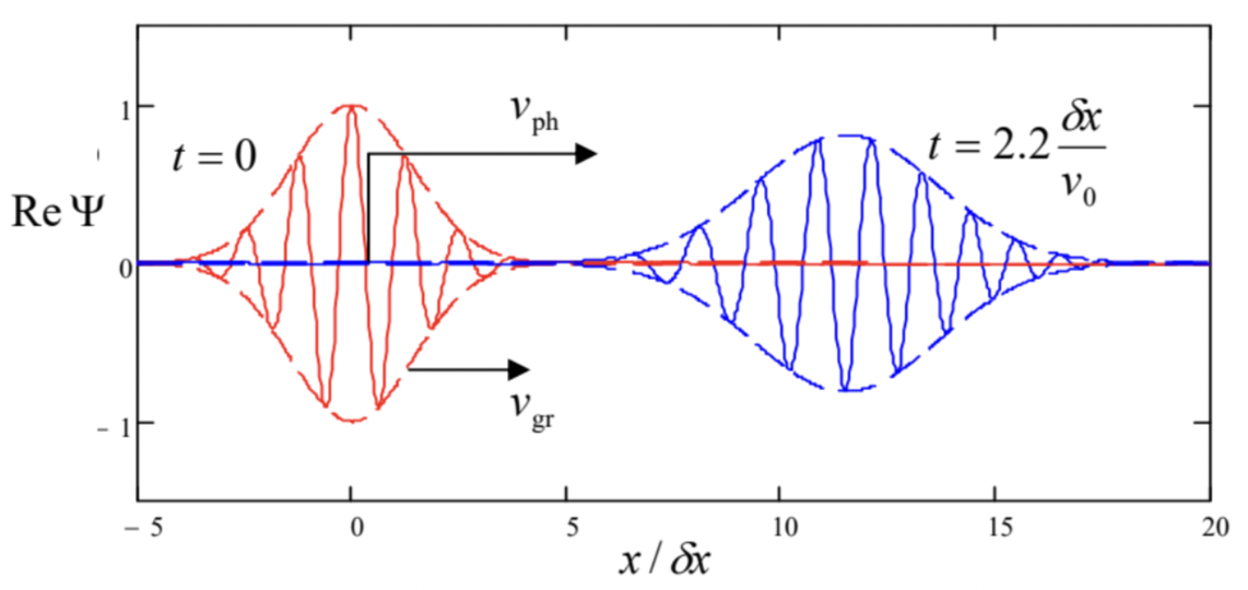
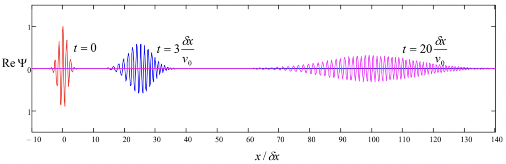
The plots clearly show the following effects:

(i) the wave packet as a whole (as characterized by its envelope) moves along the $x$-axis with a certain group velocity $v_{\mathrm{gr}}$,

(ii) the "carrier" quasi-sinusoidal wave inside the packet moves with a different, phase velocity $v_{\mathrm{ph}}$, which may be defined as the velocity of the spatial points where the wave’s phase $\varphi(x, t) \equiv \arg \Psi$ takes a certain fixed value (say, $\varphi=\pi / 2$, where $\operatorname{Re} \Psi$ vanishes), and

(iii) the wave packet’s spatial width gradually increases with time - the packet spreads.

All these effects are common for waves of any physical nature. ${ }^{7}$ Indeed, let us consider a $1 \mathrm{D}$ wave packet of the type (26), but more general: $$\Psi(x, t)=\int a_{k} e^{i(k x-\omega t)} d k,$$ propagating in a medium with an arbitrary (but smooth!) dispersion relation $\omega(k)$, and assume that the wave number distribution $a_{k}$ is narrow: $\delta k<\left\langle\langle k\rangle \equiv k_{0}-\right.$ see Fig. 1.6b. Then we may expand the function $\omega(k)$ into the Taylor series near the central wave number $k_{0}$, and keep only three of its leading terms: $$\omega(k) \approx \omega_{0}+\frac{d \omega}{d k} \widetilde{k}+\frac{1}{2} \frac{d^{2} \omega}{d k^{2}} \widetilde{k}^{2}, \quad \text { where } \widetilde{k} \equiv k-k_{0}, \omega_{0} \equiv \omega\left(k_{0}\right),$$ where both derivatives have to be evaluated at the point $k=k_{0}$. In this approximation, ${ }^{8}$ the expression in the parentheses on the right-hand side of Eq. (27) may be rewritten as $$\begin{aligned} k x-\omega(k) t & \approx k_{0} x+\widetilde{k} x-\left(\omega_{0}+\frac{d \omega}{d k} \widetilde{k}+\frac{1}{2} \frac{d^{2} \omega}{d k^{2}} \widetilde{k}^{2}\right) t \\ & \equiv\left(k_{0} x-\omega_{0} t\right)+\widetilde{k}\left(x-\frac{d \omega}{d k} t\right)-\frac{1}{2} \frac{d^{2} \omega}{d k^{2}} \widetilde{k}^{2} t \end{aligned}$$ so that Eq. (27) becomes $$\Psi(x, t) \approx e^{i\left(k_{0} x-\omega_{0} t\right)} \int a_{k} \exp \left\{i\left[\tilde{k}\left(x-\frac{d \omega}{d k} t\right)-\frac{1}{2} \frac{d^{2} \omega}{d k^{2}} \widetilde{k}^{2} t\right]\right\} d \widetilde{k}$$ First, let neglect the last term in square brackets (which is much smaller than the first term if the dispersion relation is smooth enough and/or the time interval $t$ is sufficiently small), and compare the result with the initial form of the wave packet (27): $$\Psi(x, 0)=\int a_{k} e^{i k x} d k=A(x) e^{i k_{0} x}, \quad \text { with } A(x) \equiv \int a_{k} e^{i \widetilde{k} x} d \widetilde{k}$$ The comparison shows that in this approximation, Eq. (30) is reduced to $$\Psi(x, t)=A\left(x-v_{\mathrm{gr}} t\right) e^{i k_{0}\left(x-v_{\mathrm{ph}} t\right)},$$ where $v_{\mathrm{gr}}$ and $v_{\mathrm{ph}}$ are two constants with the dimension of velocity: $$\left.v_{\mathrm{gr}} \equiv \frac{d \omega}{d k}\right|_{k=k_{0}},\left.\quad v_{\mathrm{ph}} \equiv \frac{\omega}{k}\right|_{k=k_{0}}$$ Clearly, Eq. (32) describes the effects (i) and (ii) listed above. For the particular case of the de Broglie waves, whose dispersion law is given by Eq. (1.30), $$\left.v_{\mathrm{gr}} \equiv \frac{d \omega}{d k}\right|_{k=k_{0}}=\frac{\hbar k_{0}}{m} \equiv v_{0},\left.\quad v_{\mathrm{ph}} \equiv \frac{\omega}{k}\right|_{k=k_{0}}=\frac{\hbar k_{0}}{2 m}=\frac{v_{\mathrm{gr}}}{2} .$$ We see that (very fortunately :-) the velocity of the wave packet’s envelope is equal to $v_{0}$ - the classical velocity of the same particle.

Next, the last term in the square brackets of Eq. (30) describes the effect (iii), the wave packet’s spread. It may be readily evaluated if the packet (27) is initially Gaussian, as in our example (25): $$a_{k}=\text { const } \times \exp \left\{-\frac{\widetilde{k}^{2}}{(2 \delta k)^{2}}\right\} \text {. }$$ In this case the integral (30) is Gaussian, and may be worked out exactly as the integral (21), i.e. by representing the merged exponents under the integral as a full square of a linear combination of $x$ and $k$ : $$\begin{aligned} &-\frac{\widetilde{k}^{2}}{(2 \delta k)^{2}}+i \widetilde{k}\left(x-v_{\mathrm{gr}} t\right)-\frac{i}{2} \frac{d^{2} \omega}{d k^{2}} \widetilde{k}^{2} t \\ &\equiv-\Delta(t)\left(\widetilde{k}+i \frac{x-v_{\mathrm{gr}} t}{2 \Delta(t)}\right)^{2}-\frac{\left(x-v_{\mathrm{gr}} t\right)^{2}}{4 \Delta(t)}+i k_{0} x-\frac{i}{2} \frac{d^{2} \omega}{d k^{2}} k_{0}^{2} t, \end{aligned}$$ where I have introduced the following complex function of time: $$\Delta(t) \equiv \frac{1}{4(\delta k)^{2}}+\frac{i}{2} \frac{d^{2} \omega}{d k^{2}} t=(\delta x)^{2}+\frac{i}{2} \frac{d^{2} \omega}{d k^{2}} t$$ and used Eq. (24). Now integrating over $\widetilde{k}$, we get $$\Psi(x, t) \propto \exp \left\{-\frac{\left(x-v_{\mathrm{gr}} t\right)^{2}}{4 \Delta(t)}+i\left(k_{0} x-\frac{1}{2} \frac{d^{2} \omega}{d k^{2}} k_{0}^{2} t\right)\right\} .$$ The imaginary part of the ratio $1 / \Delta(t)$ in this exponent gives just an additional contribution to the wave’s phase and does not affect the resulting probability distribution $$w(x, t)=\Psi^{*} \Psi \propto \exp \left\{-\frac{\left(x-v_{\mathrm{gr}} t\right)^{2}}{2} \operatorname{Re} \frac{1}{\Delta(t)}\right\} .$$ This is again a Gaussian distribution over axis $x$, centered to point $\langle x\rangle=v_{\text {gr }} t$, with the r.m.s. width $$\left(\delta x^{\prime}\right)^{2} \equiv\left\{\operatorname{Re}\left[\frac{1}{\Delta(t)}\right]\right\}^{-1}=(\delta x)^{2}+\left(\frac{1}{2} \frac{d^{2} \omega}{d k^{2}} t\right)^{2} \frac{1}{(\delta x)^{2}} .$$ In the particular case of de Broglie waves, $d^{2} \omega / d k^{2}=\hbar / m$, so that $$\left(\delta x^{\prime}\right)^{2}=(\delta x)^{2}+\left(\frac{\hbar t}{2 m}\right)^{2} \frac{1}{(\delta x)^{2}} .$$ The physics of the packet spreading is very simple: if $d^{2} \omega / d k^{2} \neq 0$, the group velocity $d \omega / d k$ of each small group $d k$ of the monochromatic components of the wave is different, resulting in the gradual (eventually, linear) accumulation of the differences of the distances traveled by the groups. The most curious feature of Eq. (39) is that the packet width at $t>0$ depends on its initial width $\delta x^{\prime}(0)=\delta x$ in a non-monotonic way, tending to infinity at both $\delta x \rightarrow 0$ and $\delta x \rightarrow \infty$. Because of that, for a given time interval $t$, there is an optimal value of $\delta x$ that minimizes $\delta x$ ’: $$\left(\delta x^{\prime}\right)_{\min }=\sqrt{2}(\delta x)_{o p t}=\left(\frac{\hbar t}{m}\right)^{1 / 2} .$$ This expression may be used for estimates of the spreading effect. Due to the smallness of the Planck constant $\hbar$ on the human scale of things, for macroscopic bodies this effect is extremely small even for very long time intervals; however, for light particles it may be very noticeable: for an electron $\left(m=m_{\mathrm{e}} \approx\right.$ $10^{-30} \mathrm{~kg}$ ), and $t=1 \mathrm{~s}$, Eq. (40) yields $\left(\delta x^{\prime}\right)_{\min } \sim 1 \mathrm{~cm}$.

Note also that for any $t \neq 0$, the wave packet retains its Gaussian envelope, but the ultimate relation (24) is not satisfied, $\delta x^{\prime} \delta p>\hbar / 2$ - due to a gradually accumulated phase shift between the component monochromatic waves. The last remark on this topic: in quantum mechanics, the wave packet spreading is not a ubiquitous effect! For example, in Chapter 5 we will see that in a quantum oscillator, the spatial width of a Gaussian packet (for that system, called the Glauber state of the oscillator) does not grow monotonically but rather either stays constant or oscillates in time.

Now let us briefly discuss the case when the initial wave packet is not Gaussian but is described by an arbitrary initial wavefunction. To make the forthcoming result more aesthetically pleasing, it is beneficial to generalize our calculations to an arbitrary initial time $t_{0}$; it is evident that if $U$ does not depend on time explicitly, it is sufficient to replace $t$ with $\left(t-t_{0}\right)$ in all above formulas. With this replacement, Eq. (27) becomes $$\Psi(x, t)=\int a_{k} e^{i\left[k x-\omega\left(t-t_{0}\right)\right]} d k$$ and the reciprocal transform (21) reads $$a_{k}=\frac{1}{2 \pi} \int \Psi\left(x, t_{0}\right) e^{-i k x} d x .$$ If we want to express these two formulas with one relation, i.e. plug Eq. (42) into Eq. (41), we should give the integration variable $x$ some other name, e.g., $x_{0}$. (Such notation is appropriate because this variable describes the coordinate argument in the initial wave packet.) The result is $$\Psi(x, t)=\frac{1}{2 \pi} \int d k \int d x_{0} \Psi\left(x_{0}, t_{0}\right) e^{i\left[k\left(x-x_{0}\right)-\omega\left(t-t_{0}\right)\right]} .$$ Changing the order of integration, this expression may be rewritten in the following general form: $$\Psi(x, t)=\int G\left(x, t ; x_{0}, t_{0}\right) \Psi\left(x_{0}, t_{0}\right) d x_{0},$$ where the function $G$, usually called kernel in mathematics, in quantum mechanics is called the propagator. ${ }^{9}$ Its physical sense may be understood by considering the following special initial condition: ${ }^{10}$ $$\Psi\left(x_{0}, t_{0}\right)=\delta\left(x_{0}-x^{\prime}\right),$$ where $x$ ’ is a certain point within the domain of particle’s motion. In this particular case, Eq. (44) gives $$\Psi(x, t)=G\left(x, t ; x^{\prime}, t_{0}\right) .$$ Hence, the propagator, considered as a function of its arguments $x$ and $t$ only, is just the wavefunction of the particle, at the $\delta$-functional initial conditions (45). Thus just as Eq. (41) may be understood as a mathematical expression of the linear superposition principle in the momentum (i.e., reciprocal) space domain, Eq. (44) is an expression of this principle in the direct space domain: the system’s "response" $\Psi(x, t)$ to an arbitrary initial condition $\Psi\left(x_{0}, t_{0}\right)$ is just a sum of its responses to its elementary spatial "slices" of this initial function, with the propagator $G\left(x, t ; x_{0}, t_{0}\right)$ representing the weight of each slice in the final sum.

According to Eqs. (43) and (44), in the particular case of a free particle the propagator is equal to $$G\left(x, t ; x_{0}, t_{0}\right)=\frac{1}{2 \pi} \int e^{i\left[k\left(x-x_{0}\right)-\omega\left(t-t_{0}\right)\right]} d k,$$ Calculating this integral, one should remember that here $\omega$ is not a constant but a function of $k$, given by the dispersion relation for the partial waves. In particular, for the de Broglie waves, with $\hbar \omega=\hbar^{2} k^{2} / 2 m$, $$G\left(x, t ; x_{0}, t_{0}\right) \equiv \frac{1}{2 \pi} \int \exp \left\{i\left[k\left(x-x_{0}\right)-\frac{\hbar k^{2}}{2 m}\left(t-t_{0}\right)\right]\right\} d k \text {. }$$ This is a Gaussian integral again, and may be readily calculated just it was done (twice) above, by completing the exponent to the full square. The result is $$G\left(x, t ; x_{0}, t_{0}\right)=\left(\frac{m}{2 \pi i \hbar\left(t-t_{0}\right)}\right)^{1 / 2} \exp \left\{-\frac{m\left(x-x_{0}\right)^{2}}{2 i \hbar\left(t-t_{0}\right)}\right\} .$$ Please note the following features of this complex function (plotted in Fig. 2):

(i) It depends only on the differences $\left(x-x_{0}\right)$ and $\left(t-t_{0}\right)$. This is natural because the free-particle propagation problem is translation-invariant both in space and time.

(ii) The function’s shape does not depend on its arguments - they just rescale the same function: its snapshot (Fig. 2), if plotted as a function of un-normalized $x$, just becomes broader and lower with time. It is curious that the spatial broadening scales as $\left(t-t_{0}\right)^{1 / 2}-$ just as at the classical diffusion, as a result of a deep mathematical analogy between quantum mechanics and classical statistics - to be discussed further in Chapter $7 .$

(iii) In accordance with the uncertainty relation, the ultimately compressed wave packet (45) has an infinite width of momentum distribution, and the quasi-sinusoidal tails of the free-particle propagator, clearly visible in Fig. 2, are the results of the free propagation of the fastest (highestmomentum) components of that distribution, in both directions from the packet center.

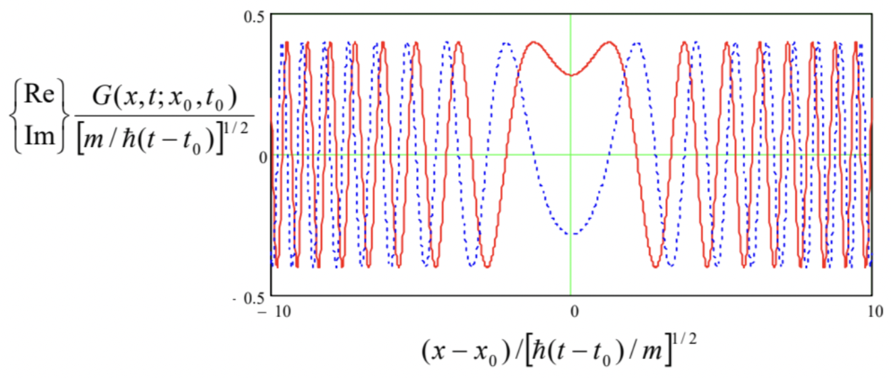Fig. 2.2. The real (solid line) and imaginary (dotted line) parts of the 1D free particle’s propagator (49).

In the following sections, I will mostly focus on monochromatic wavefunctions (that, for unconfined motion, may be interpreted as wave packets of a very large spatial width $\delta x$ ), and only rarely discuss wave packets. My best excuse is the linear superposition principle, i.e. our conceptual ability to restore the general solution from that of monochromatic waves of all possible energies. However, the reader should not forget that, as the above discussion has illustrated, mathematically such restoration is not always trivial.

---

${ }^{2}$ From this point on to the end of this chapter, I will drop the index $x$ in the $x$-components of the vectors $\mathbf{k}$ and $\mathbf{p}$.

${ }^{3}$ This fact may be readily proven using the well-known integral of the Gaussian function (17), in infinite limits see, e.g., MA Eq. (6.9b). It is also straightforward to use MA Eq. (6.9c) to prove that for the wave packet (16), the parameter $\delta x$ is indeed the r.m.s. uncertainty (1.34) of the coordinate $x$, thus justifying its notation.

${ }^{4}$ For the notation brevity, from this point on the infinite limit signs will be dropped in all 1D integrals.

${ }^{5}$ The fact that the argument’s shift is imaginary is not important. Indeed, since the function under the integral tends to zero at Re $x^{\prime} \equiv \operatorname{Re} x \rightarrow \pm \infty$, the difference between infinite integrals of this function along axes of $x$ and $x^{\prime}$ is equal to its contour integral around the rectangular area $x \leq \operatorname{Im} z \leq x$ ’. Since the function is also analytical, it obeys the Cauchy theorem MA Eq. (15.1), which says that this contour integral equals zero.

${ }^{6}$ Note that Eq. (26) differs from Eq. (16) only by an exponent of a purely imaginary number, and hence this wavefunction is also properly normalized to 1 - see Eq. (3). Hence the wave packet introduction offers a natural solution to the problem of traveling de Broglie wave’s normalization, which was mentioned in Sec. 1.2.

${ }^{7}$ See, e.g., brief discussions in CM Sec. $6.3$ and EM Sec. $7.2$.

${ }^{8}$ By the way, in the particular case of de Broglie waves described by the dispersion relation (1.30), Eq. (28) is exact, because $\omega=E / \hbar$ is a quadratic function of $k=p / \hbar$, and all higher derivatives of $\omega$ over $k$ vanish for any $k_{0}$.

${ }^{9}$ Its standard notation by letter $G$ stems from the fact that the propagator is essentially the spatial-temporal Green’s function, defined very similarly to Green’s functions of other ordinary and partial differential equations describing various physics systems - see, e.g., CM Sec. $5.1$ and/or EM Sec. $2.7$ and 7.3.

${ }^{10}$ Note that such initial condition is mathematically not equivalent to a $\delta$-functional initial probability density (3).