2.7: 2.6. Localized State Coupling, and Quantum Oscillations

Now let us discuss one more effect specific to quantum mechanics. Its mathematical description may be simplified using a model potential consisting of two very short and deep potential wells. For that, let us first analyze the properties of a single well of this type (Fig. 18), which may be modeled similarly to the short and high potential barrier - see Eq. (74), but with a negative "weight": \[U(x)=-w \delta(x), \quad \text { with } w>0 .\]

In contrast to its tunnel-barrier counterpart (74), such potential sustains a stationary state with a negative eigenenergy \(E<0\), and a localized eigenfunction \(\psi\), with \(|\psi| \rightarrow 0\) at \(x \rightarrow \pm \infty\).

Fig. \(2.18\). Delta-functional potential well and its localized eigenstate (schematically).

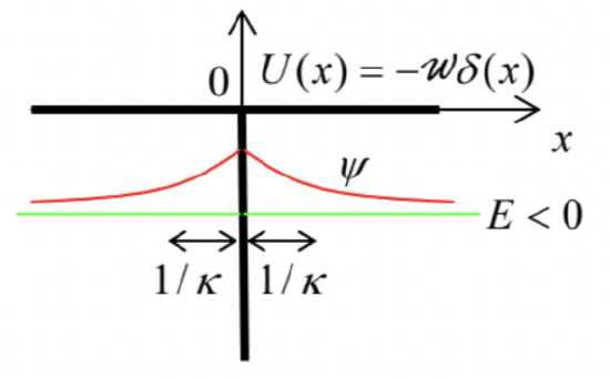
Indeed, at \(x \neq 0, U(x)=0\), so the \(1 \mathrm{D}\) Schrödinger equation is reduced to the Helmholtz equation (1.83), whose localized solutions with \(E<0\) are single exponents, vanishing at large distances: \({ }^{38}\) \[\psi(x)=\psi_{0}(x) \equiv\left\{\begin{array}{ll} A e^{-\kappa x}, & \text { for } x>0, \\ A e^{+\kappa x}, & \text { for } x<0, \end{array} \quad \text { with } \frac{\hbar^{2} \kappa^{2}}{2 m}=-E, \quad \kappa>0 .\right.\] (The coefficients before the exponents have been selected equal to satisfy the boundary condition (76) of the wavefunction’s continuity at \(x=0\).) Plugging Eq. (159) into the second boundary condition, given by Eq. (75), but now with the negative sign before \(w\), we get \[(-\kappa A)-(+\kappa A)=-\frac{2 m w}{\hbar^{2}} A,\] in which the common factor \(A \neq 0\) may be canceled. This equation \({ }^{39}\) has one solution for any \(w>0\) : \[\kappa=\kappa_{0} \equiv \frac{m w}{\hbar^{2}},\] and hence the system has only one (ground) localized state, with the following eigenenergy: 40 \[E=E_{0} \equiv-\frac{\hbar^{2} \kappa_{0}^{2}}{2 m}=-\frac{m w^{2}}{2 \hbar^{2}} .\] Now we are ready to analyze localized states of the two-well potential shown in Fig. 19: \[U(x)=-w\left[\delta\left(x-\frac{a}{2}\right)+\delta\left(x+\frac{a}{2}\right)\right], \quad \text { with } w>0 .\] Here we may still use the single-exponent solutions, similar to Eq. (159), for the wavefunction outside the interval \([-a / 2,+a / 2]\), but inside the interval, we need to take into account both possible exponents: \[\psi=C_{+} e^{\kappa x}+C_{-} e^{-\kappa x} \equiv C_{\mathrm{A}} \sinh \kappa x+C_{\mathrm{S}} \cosh \kappa x, \quad \text { for }-\frac{a}{2} \leq x \leq+\frac{a}{2},\] with the parameter \(\kappa\) defined as in Eq. (159). The last of these equivalent expressions is more convenient because due to the symmetry of the potential (163) to the central point \(x=0\), the system’s eigenfunctions should be either symmetric (even) or antisymmetric (odd) functions of \(x\) (see Fig. 19), so that they may be analyzed separately, only for one half of the system, say \(x \geq 0\), and using just one of the hyperbolic function (164) in each case.

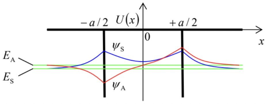Fig. 2.19. A system of two coupled potential wells, and its localized eigenstates (schematically).

For the antisymmetric eigenfunction, Eqs. (159) and (164) yield \[\psi_{\mathrm{A}} \equiv C_{\mathrm{A}} \times\left\{\begin{array}{lr} \sinh \kappa x, & \text { for } 0 \leq x \leq \frac{a}{2}, \\ \sinh \frac{\kappa a}{2} \exp \left\{-\kappa\left(x-\frac{a}{2}\right)\right\}, & \text { for } \frac{a}{2} \leq x, \end{array}\right.\] where the front coefficient in the lower line has been selected to satisfy the condition (76) of the wavefunction’s continuity at \(x=+a / 2-\) and hence at \(x=-a / 2\). What remains is to satisfy the condition (75), with a negative sign before \(w\), for the derivative’s jump at that point. This condition yields the following characteristic equation: \[\sinh \frac{\kappa a}{2}+\cosh \frac{\kappa a}{2}=\frac{2 m w}{\hbar^{2} \kappa} \sinh \frac{\kappa a}{2}, \quad \text { i.e. } 1+\operatorname{coth} \frac{\kappa a}{2}=2 \frac{\left(\kappa_{0} a\right)}{(\kappa a)},\] where \(\kappa_{0}\), given by Eq. (161), is the value of \(\kappa\) for a single well, i.e. the reciprocal spatial width of its localized eigenfunction - see Fig. 18 .

Figure 20 a shows both sides of Eq. (166) as functions of the dimensionless product \(\kappa a\), for several values of the parameter \(\kappa_{0} a\), i.e. of the normalized distance between the two wells. The plots show, first of all, that as the parameter \(\kappa_{0} a\) is decreased, the LHS and RHS plots cross (i.e. Eq. (166) has a solution) at lower and lower values of \(\kappa a\). At \(\kappa a<<1\), the left-hand side of the last form of this equation may be approximated as \(2 / \kappa a\). Comparing this expression with the right-hand side of the characteristic equation, we see that this transcendental equation has a solution (i.e. the system has an antisymmetric localized state) only if \(\kappa_{0} a>1\), i.e. if the distance \(a\) between the two narrow potential wells is larger than the following value, \[a_{\min }=\frac{1}{\kappa_{0}} \equiv \frac{\hbar^{2}}{m w},\] which is equal to the characteristic spread of the wavefunction in a single well - see Fig. 18. (At \(a \rightarrow\) \(a_{\min }, \kappa a \rightarrow 0\), meaning that the state’s localization becomes weaker and weaker.)

(a) the antisymmetric eigenstate (165), and (b) the symmetric eigenstate (171).

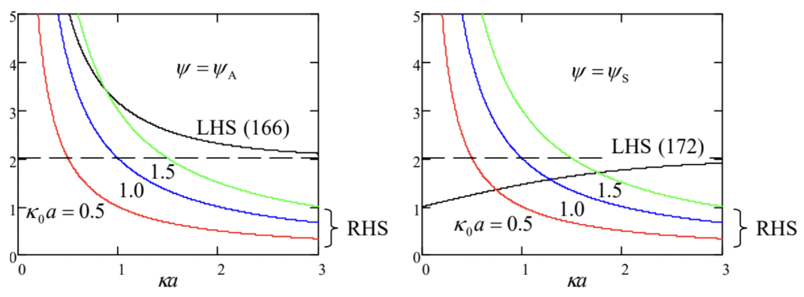
In the opposite limit of large distances between the potential wells, i.e. \(\kappa_{0} a \gg 1\), Eq. (166) shows that \(\kappa a>>1\) as well, so that its left-hand side may be approximated as \(2(1+\exp \{-\kappa a\})\), and the equation yields \[\kappa \approx \kappa_{0}\left(1-\exp \left\{-\kappa_{0} a\right\}\right) \approx \kappa_{0} .\] This result means that the eigenfunction is an antisymmetric superposition of two virtually unperturbed wavefunctions (159) of each partial potential well: \[\psi_{\mathrm{A}}(x) \approx \frac{1}{\sqrt{2}}\left[\psi_{\mathrm{R}}(x)-\psi_{\mathrm{L}}(x)\right], \quad \text { where } \psi_{\mathrm{R}}(x) \equiv \psi_{0}\left(x-\frac{a}{2}\right), \quad \psi_{\mathrm{L}}(x) \equiv \psi_{0}\left(x+\frac{a}{2}\right),\] and the front coefficient is selected in such a way that if the eigenfunction \(\psi_{0}\) of each well is normalized, so is \(\psi_{\mathrm{A}}\). Plugging the middle (more exact) form of Eq. (168) into the last of Eqs. (159), we can see that in this limit the antisymmetric state’s energy is only slightly higher than the eigenenergy \(E_{0}\) of a single well, given by Eq. (162): \[E_{\mathrm{A}} \approx E_{0}\left(1-2 \exp \left\{-\kappa_{0} a\right\}\right) \equiv E_{0}+\delta, \quad \text { where } \delta \equiv \frac{2 m w^{2}}{\hbar^{2}} \exp \left\{-\kappa_{0} a\right\}>0 .\] The symmetric eigenfunction has a form reminding Eq. (165), but still different from it: \[\psi=\psi_{\mathrm{S}} \equiv C_{\mathrm{S}} \times\left\{\begin{array}{lr} \cosh \kappa x, & \text { for } 0 \leq x \leq \frac{a}{2}, \\ \cosh \frac{\kappa a}{2} \exp \left\{-\kappa\left(x-\frac{a}{2}\right)\right\}, & \text { for } \frac{a}{2} \leq x, \end{array}\right.\] giving a characteristic equation similar in structure to Eq. (166), but with a different left-hand side: \[1+\tanh \frac{\kappa a}{2}=2 \frac{\left(\kappa_{0} a\right)}{(\kappa a)} \text {. }\] Figure \(20 \mathrm{~b}\) shows both sides of this equation for several values of the parameter \(\kappa_{0} a\). It is evident that in contrast to Eq. (166), Eq. (172) has a unique solution (and hence the system has a localized symmetric eigenstate) for any value of the parameter \(\kappa_{0} a\), i.e. for any distance between the partial wells. In the limit of very close wells (i.e. their strong coupling), \(\kappa_{0} a<<1\), we get \(\kappa a<<1\), \(\tanh (\kappa a / 2) \rightarrow 0\), and Eq. (172) yields \(\kappa \rightarrow 2 \kappa_{0}\), leading to a four-fold increase of the eigenenergy’s magnitude in comparison with that of the single well: \[E_{\mathrm{S}} \approx 4 E_{0} \equiv-\frac{m(2 w)^{2}}{2 \hbar^{2}}, \quad \text { for } \kappa_{0} a<<1 .\] The physical meaning of this result is very simple: two very close potential wells act (on the symmetric eigenfunction only!) together, so that their "weights" \(w \equiv \int U(x) d x\) just add up.

In the opposite, weak coupling limit, i.e. \(\kappa_{0} a>>1\), Eq. (172) shows that \(\kappa a>>1\) as well, so that its left-hand side may be approximated as \(2(1-\exp \{-\kappa a\})\), and the equation yields \[\kappa \approx \kappa_{0}\left(1+\exp \left\{-\kappa_{0} a\right\}\right) \approx \kappa_{0} .\] In this limit, the eigenfunction is a symmetric superposition of two virtually unperturbed wavefunctions (159) of each partial potential well: \[\psi_{\mathrm{S}}(x) \approx \frac{1}{\sqrt{2}}\left[\psi_{\mathrm{R}}(x)+\psi_{\mathrm{L}}(x)\right],\] and the eigenenergy is also close to the energy \(E_{0}\) of a partial well, but is slightly lower: \[E_{\mathrm{S}} \approx E_{0}\left(1+2 \exp \left\{-\kappa_{0} a\right\}\right) \equiv E_{0}-\delta, \quad \text { so that } E_{\mathrm{A}}-E_{\mathrm{S}}=2 \delta,\] where \(\delta\) is again given by the last of Eqs. (170).

So, the eigenenergy of the symmetric state is always lower than that of the antisymmetric state. The physics of this effect (which remains qualitatively the same in more complex two-component systems, most importantly in diatomic molecules such as \(\mathrm{H}_{2}\) ) is evident from the sketch of the wavefunctions \(\psi_{\mathrm{A}}\) and \(\psi_{\mathrm{s}}\), given by Eqs. (165) and (171), in Fig. 19. In the antisymmetric mode, the wavefunction has to vanish at the center of the system, so that each its half is squeezed to one half of the system’s spatial extension. Such a squeeze increases the function’s gradient, and hence its kinetic energy (1.27), and hence its total energy. On the contrary, in the symmetric mode, the wavefunction effectively spreads into the counterpart well. As a result, it changes in space slower, and hence its kinetic energy is also lower.

Even more importantly, the symmetric state’s energy decreases as the distance \(a\) is decreased, corresponding to the effective attraction of the partial wells. This is a good toy model of the strongest (and most important) type of atomic cohesion - the covalent (or "chemical") bonding. \({ }^{41}\) In the simplest case of the \(\mathrm{H}_{2}\) molecule, each of two electrons of the system, in its ground state, \({ }^{42}\) reduces its kinetic energy by spreading its wavefunction around both hydrogen nuclei (protons), rather than being confined near one of them - as it had to be in a single atom. The resulting bonding is very strong: in chemical units, \(429 \mathrm{~kJ} / \mathrm{mol}\), i.e. \(18.6 \mathrm{eV}\) per molecule. Perhaps counter-intuitively, this quantum-mechanical covalent bonding is even stronger than the strongest classical (ionic) bonding due to electron transfer between atoms, leading to the Coulomb attraction of the resulting ions. (For example, the atomic cohesion in the \(\mathrm{NaCl}\) molecule is just \(3.28 \mathrm{eV}\).)

Now let us analyze the dynamic properties of our model system (Fig. 19) because such a pair of weakly coupled potential wells is our first example of the very important class of two-level systems. \({ }^{43}\) It is easiest to do in the weak-coupling limit \(\kappa_{0} a>>1\), when the simple results (168)-(170) and (174)-(176) are quantitatively valid. In particular, Eqs. (169) and (175) enable us to represent the quasi-localized states of the particle in each partial well as linear combinations of its two eigenstates: \[\psi_{\mathrm{R}}(x)=\frac{1}{\sqrt{2}}\left[\psi_{\mathrm{S}}(x)+\psi_{\mathrm{A}}(x)\right], \quad \psi_{\mathrm{L}}(x)=\frac{1}{\sqrt{2}}\left[\psi_{\mathrm{S}}(x)-\psi_{\mathrm{A}}(x)\right] .\] Let us perform the following thought ("gedanken") experiment: place a particle, at \(t=0\), into one of these quasi-localized states, say \(\psi_{\mathrm{R}}(x)\), and leave the system alone to evolve, so that \[\Psi(x, 0)=\psi_{\mathrm{R}}(x)=\frac{1}{\sqrt{2}}\left[\psi_{\mathrm{S}}(x)+\psi_{\mathrm{A}}(x)\right] .\] According to the general solution (1.69) of the time-independent Schrödinger equation, the time dynamics of this wavefunction may be obtained simply by multiplying each eigenfunction by the corresponding complex-exponential time factor: \[\Psi(x, t)=\frac{1}{\sqrt{2}}\left[\psi_{\mathrm{S}}(x) \exp \left\{-i \frac{E_{\mathrm{S}}}{\hbar} t\right\}+\psi_{\mathrm{A}}(x) \exp \left\{-i \frac{E_{\mathrm{A}}}{\hbar} t\right\}\right] .\] From here, using Eqs. (170) and (176), and then Eqs. (169) and (175) again, we get \[\begin{aligned} \Psi(x, t) &=\frac{1}{\sqrt{2}}\left(\psi_{\mathrm{S}}(x) \exp \left\{\frac{i \delta t}{\hbar}\right\}+\psi_{\mathrm{A}}(x) \exp \left\{-\frac{i \delta t}{\hbar}\right\}\right) \exp \left\{-\frac{i E_{0} t}{\hbar}\right\} \\ & \equiv\left(\psi_{\mathrm{R}}(x) \cos \frac{\delta t}{\hbar}+i \psi_{\mathrm{L}}(x) \sin \frac{\delta t}{\hbar}\right) \exp \left\{-i \frac{E_{0} t}{\hbar}\right\} . \end{aligned}\] This result implies, in particular, that the probabilities \(W_{\mathrm{R}}\) and \(W_{\mathrm{L}}\) to find the particle, respectively, in the right and left wells change with time as \[W_{\mathrm{R}}=\cos ^{2} \frac{\delta t}{\hbar}, \quad W_{\mathrm{L}}=\sin ^{2} \frac{\delta t}{\hbar},\] mercifully leaving the total probability constant: \(W_{\mathrm{R}}+W_{\mathrm{L}}=1\). (If our calculation had not passed this sanity check, we would be in big trouble.)

This is the famous effect of quantum oscillations \(^{44}\) of the particle’s wavefunction between two similar, coupled subsystems, with the frequency \[\omega=\frac{2 \delta}{\hbar} \equiv \frac{E_{\mathrm{A}}-E_{\mathrm{S}}}{\hbar} .\] In its last form, this result does not depend on the assumption of weak coupling, though the simple form (181) of the oscillations, with its \(100 \%\) probability variations, does. (Indeed, at a strong coupling of two subsystems, the very notion of the quasi-localized states \(\psi_{\mathrm{R}}\) and \(\psi_{\mathrm{L}}\) is ambiguous.) Qualitatively, this effect may be interpreted as follows: the particle, placed into one of the potential wells, tries to escape from it via tunneling through the potential barrier separating the wells. (In our particular system, shown in Fig. 17, the barrier is formed by the spatial segment of length \(a\), which has the potential energy, \(U=\) 0 , higher than the eigenstate energy \(-E_{0}\).) However, in the two-well system, the particle can only escape into the adjacent well. After the tunneling into that counterpart well, the particle tries to escape from it, and hence comes back, etc. - very much as a classical 1D oscillator, initially deflected from its equilibrium position, at negligible damping.

Some care is required at using such interpretation for quantitative conclusions. In particular, let us compare the period \(\tau \equiv 2 \pi / \omega\) of the oscillations (181) with the metastable state’s lifetime discussed in the previous section. For our particular model, we may use the second of Eqs. (170) to write \[\omega=\frac{4\left|E_{0}\right|}{\hbar} \exp \left\{-\kappa_{0} a\right\}, \quad \tau=\frac{\pi \hbar}{\delta}=\frac{\pi \hbar}{2\left|E_{0}\right|} \exp \left\{\kappa_{0} a\right\} \equiv \frac{t_{\mathrm{a}}}{2} \exp \left\{\kappa_{0} a\right\}, \quad \text { for } \kappa_{0} a>>1,\] where \(t_{\mathrm{a}} \equiv 2 \pi / \omega_{0} \equiv 2 \pi \hbar /\left|E_{0}\right|\) is the effective attempt time. On the other hand, according to Eq. (80), the transparency \(\mathscr{T}\) of our potential barrier, in this limit, scales as \(\exp \left\{-2 \kappa_{0} a\right\},{ }^{45}\) so that according to the general relation (153), the lifetime \(\tau\) is of the order of \(t_{\mathrm{a}} \exp \left\{2 \kappa_{0} a\right\} \gg T\). This is a rather counterintuitive result: the speed of particle tunneling into a similar adjacent well is much higher than that, through a similar barrier, to the free space!In order to show that this important result is not an artifact of our delta-functional model of the potential barrier, and also compare \(\tau\) and \(\tau\) more directly, let us analyze the quantum oscillations between two weakly coupled wells, now assuming that the (symmetric) potential profile \(U(x)\) is sufficiently soft (Fig. 21), so that all its eigenfunctions \(\psi_{\mathrm{S}}\) and \(\psi_{\mathrm{A}}\) are at least differentiable at all points. \({ }^{46}\) If the barrier’s transparency is low, the quasi-localized wavefunctions \(\psi_{\mathrm{R}}(x)\) and \(\psi_{\mathrm{L}}(x)=\psi_{\mathrm{R}}(-x)\) and their eigenenergies may be found approximately by solving the Schrödinger equations in one of the wells, neglecting the tunneling through the barrier, but the calculation of \(\delta\) requires a little bit more care. Let us write the stationary Schrödinger equations for the symmetric and antisymmetric solutions in the form \[\left[E_{\mathrm{A}}-U(x)\right] \psi_{\mathrm{A}}=-\frac{\hbar^{2}}{2 m} \frac{d^{2} \psi_{\mathrm{A}}}{d x^{2}}, \quad\left[E_{\mathrm{S}}-U(x)\right] \psi_{\mathrm{S}}=-\frac{\hbar^{2}}{2 m} \frac{d^{2} \psi_{\mathrm{S}}}{d x^{2}},\] multiply the former equation by \(\psi_{\mathrm{S}}\) and the latter one by \(\psi_{\mathrm{A}}\), subtract them from each other, and then integrate the result from 0 to \(\infty\). The result is \[\left(E_{\mathrm{A}}-E_{\mathrm{S}}\right) \int_{0}^{\infty} \psi_{\mathrm{S}} \psi_{\mathrm{A}} d x=\frac{\hbar^{2}}{2 m} \int_{0}^{\infty}\left(\frac{d^{2} \psi_{\mathrm{S}}}{d x^{2}} \psi_{\mathrm{A}}-\frac{d^{2} \psi_{\mathrm{A}}}{d x^{2}} \psi_{\mathrm{S}}\right) d x .\] If \(U(x)\), and hence \(d^{2} \psi_{\mathrm{A}, \mathrm{S}} / d x^{2}\), are finite for all \(x\), we may integrate the right-hand side by parts to get \[\left(E_{\mathrm{A}}-E_{\mathrm{S}}\right) \int_{0}^{\infty} \psi_{\mathrm{S}} \psi_{\mathrm{A}} d x=\frac{\hbar^{2}}{2 m}\left(\frac{d \psi_{\mathrm{S}}}{d x} \psi_{\mathrm{A}}-\frac{d \psi_{\mathrm{A}}}{d x} \psi_{\mathrm{S}}\right)_{0}^{\infty}\]

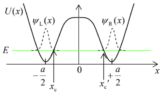Fig. 2.21. Weak coupling between two similar, soft potential wells.

So far, this result is exact (provided that the derivatives participating in it are finite at each point); for weakly coupled wells, it may be further simplified. Indeed, in this case, the left-hand side of Eq. (186) may be approximated as \[\left(E_{\mathrm{A}}-E_{\mathrm{S}}\right) \int_{0}^{\infty} \psi_{\mathrm{S}} \psi_{\mathrm{A}} d x \approx \frac{E_{\mathrm{A}}-E_{\mathrm{S}}}{2} \equiv \delta,\] because this integral is dominated by the vicinity of point \(x=a / 2\), where the second terms in each of Eqs. (169) and (175) are negligible, and the integral is equal to \(1 / 2\), assuming the proper normalization of the function \(\psi_{\mathrm{R}}(x)\). On the right-hand side of Eq. (186), the substitution at \(x=\infty\) vanishes (due to the wavefunction’s decay in the classically forbidden region), and so does the first term at \(x=0\), because for the antisymmetric solution, \(\psi_{\mathrm{A}}(0)=0\). As a result, the energy half-split \(\delta\) may be expressed in any of the following (equivalent) forms: \[\delta=\frac{\hbar^{2}}{2 m} \psi_{\mathrm{S}}(0) \frac{d \psi_{\mathrm{A}}}{d x}(0)=\frac{\hbar^{2}}{m} \psi_{\mathrm{R}}(0) \frac{d \psi_{\mathrm{R}}}{d x}(0)=-\frac{\hbar^{2}}{m} \psi_{\mathrm{L}}(0) \frac{d \psi_{\mathrm{L}}}{d x}(0) .\] It is straightforward (and hence left for the reader’s exercise) to show that within the limits of the WKB approximation’s validity, Eq. (188) may be reduced to \[\delta=\frac{\hbar}{t_{\mathrm{a}}} \exp \left\{-\int_{x_{\mathrm{c}}}^{x_{\mathrm{c}}^{\prime}} \kappa\left(x^{\prime}\right) d x^{\prime}\right\}, \quad \text { so that } \tau \equiv \frac{\pi \hbar}{\delta}=\frac{t_{\mathrm{a}}}{2} \exp \left\{\int_{x_{\mathrm{c}}}^{x_{\mathrm{c}}^{\prime}} \kappa\left(x^{\prime}\right) d x^{\prime}\right\}\] where \(t_{\mathrm{a}}\) is the time period of the classical motion of the particle, with the energy \(E \approx E_{\mathrm{A}} \approx E_{\mathrm{S}}\), inside each well, the function \(\kappa(x)\) is defined by Eq. (82), and \(x_{\mathrm{c}}\) and \(x_{\mathrm{c}}\) ’ are the classical turning points limiting the potential barrier at the level \(E\) of the particle’s eigenenergy - see Fig. 21. The result (189) is evidently a natural generalization of Eq. (183), so that the strong relationship between the times of particle tunneling into the continuum of states and into a discrete eigenstate, is indeed not specific for the delta-functional model. We will return to this fact, in its more general form, at the end of Chapter 6.

---

\({ }^{38}\) See Eqs. (56)-(58), with \(U_{0}=0\).

\({ }^{39}\) Such algebraic equations for linear differential equations are frequently called characteristic.

\({ }^{40}\) Note that this \(E_{0}\) is equal, by magnitude, to the constant \(E_{0}\) that participates in Eq. (79). Note also that this result was actually already obtained, "backward", in the solution of Problem 1.12(ii), but that solution did not address the issue of whether the calculated potential (158) could sustain any other localized eigenstates.

\({ }^{41}\) Historically, the development of the quantum theory of such bonding in the \(\mathrm{H}_{2}\) molecule (by Walter Heinrich Heitler and Fritz Wolfgang London in 1927) was the breakthrough decisive for the acceptance of the thenemerging quantum mechanics by the community of chemists.

\({ }^{42}\) Due to the opposite spins of these electrons, the Pauli principle allows them to be in the same orbital ground state - see Chapter 8 .

\({ }^{43}\) As we will see later in Chapter 4 , these properties are similar to those of spin- \(1 / 2\) particles; hence two-level systems are frequently called the spin-1/2-like systems.

\({ }^{44}\) Sometimes they are called the Bloch oscillations, but more commonly the last term is reserved for a related but different effect in spatially-periodic systems - to be discussed in Sec. 8 below.

\({ }^{45}\) It is hard to use Eq. (80) for a more exact evaluation of \(\mathscr{T}\) in our current system, with its infinitely deep potential wells, because the meaning of the wave number \(k\) is not quite clear. However, this is not too important, because in the limit \(\kappa_{0} a \gg 1\), the tunneling exponent makes the dominant contribution into the transparency see, again, Fig. 2.7b.

\({ }^{46}\) Such a smooth well may have more than one quasi-localized eigenstate, so that the proper state (and energy) index \(n\) is implied in all remaining formulas of this section.